This document summarizes artificial neural networks (ANN), which were inspired by biological neural networks in the human brain. ANNs consist of interconnected computational units that emulate neurons and pass signals to other units through connections with variable weights. ANNs are arranged in layers and learn by modifying the weights between units based on input and output data to minimize error. Common ANN algorithms include backpropagation for supervised learning to predict outputs from inputs.

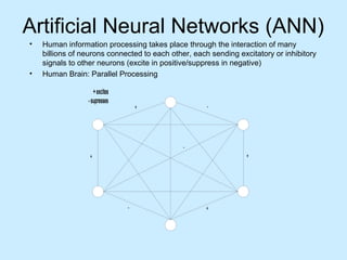
1. Artificial Neural Networks (ANN)
• Human information processing takes place through the interaction of many
billions of neurons connected to each other, each sending excitatory or inhibitory
signals to other neurons (excite in positive/suppress in negative)
• Human Brain: Parallel Processing
+ excites
- supresses
+ -
-
+ +
- +

2. ANN
• The neuron receives signals from other
neurons, collects the input signals, and
transforms the collected input signal
• The single neuron then transmits the
transformed signal to other neurons

3. ANN
• The signals that pass through the junction, known as synapses, are
either weakened or strengthened depending upon the strength of the
synaptic connection
• By modifying synaptic strengths, the human brain is able to store
knowledge and thus allow certain inputs to result in specific output or
behavior
• Translates into a mathematical model
• Artificial Neural Networks compare weights
– Synopsis is small = -
– Synopsis is large = +
• ON = +
• OFF = -
• Neurons are trained
– Neurons are on (+) or off (-)
• Example: Could be Facial Recognition

4. ANN
• A basic ANN model consists of
– Computational units
– Links
• A unit emulate the functions of a neuron
• Computational units are connected by links with
variable weights which represent synapses in the
biological model (Human Brain)
• Learning Curve: Change synopsis in face recognition
– Changes & learns new info

5. ANN
• The unit receives a weighted sum of all
its input via connections and computes
its own output value using its own
output function
• The output value is then propagated to
many other units via connection
between units

6. Basic Representation
• Parallel Transfer
– Some connections bi-directional, some one-way
• Variation of algorithms
– 2 levels
– Multi-levels
• y=f (x1, x2, x3)
– where is is a transform function (linear or non-linear)

7. Basic Representation
Sum: Netj = Sum of Wji Xi
Transfer: Yj = F (Netj )
S u m Transfer
X1
X2
X3 jth Computational
Unit
Weights
Wj1
Wj2
Wj3
Yj
Output Path

8. ANN
• Computational units in ANN are
arranged in layers - input, output, and
hidden layers
• Units in a hidden layer are called
hidden units

9. Hidden Units
• Hidden unit is a unit which represents
neither input nor output variables
• It is used to support the required
function from input to output

13. ANN Learning Algorithm
Supervised Learning Unsupervised Learning
Binary Input Continued Binary Continued
Hopfield Net Perceptron ART I ART II
Boltzman- Backpropagation Self-organizing
Machine (popular algorithm widely used) Map

14. Backpropagation
• The algorithm is a learning rule which
suggests a way of modifying weights to
represent a function from input to output
• The network architecture is a
feedforward network where
computational units are structured in a
multi-layered network: an input layer,
one or more hidden layer(s), and an
output layer

15. Backpropagation
• The units on a layer have full
connections to units on the adjacent
layers, but no connection to units on the
same layer

16. Backpropagation
• Calculate the difference (error) between
the expected and actual output value
• Adjust the weights in order to minimize
the error
• Minimize the error by performing a
gradient decent on the error surface

17. Backpropagation
• The amount of the weight change for
each input pattern in an epoch is
proportional to the error
• An epoch is completed after the
network sees all of the input and output
pairs

18. Five Input Var.
Net Working Capital/Total Assets
Retained Earning/Total Assets
EBIT/Total Assets
Market Value of Common
and Preferred Stock/Book Value
of Debt
Sales/Total Assets
Two Output Variables
Solvent Firms
Bankrupt Firms
An ANN model to Predict a Firm’s Bankruptcy

19. Advantages of ANN
• Parallel Processing
• Generalization
– a great deal of noise and randomness can
be tolerated
• Fault tolerance
– damage to a few units and weights may
not be fatal to the overall network
performance

20. Properties of ANN
• No special recovery mechanism is
required for incomplete information
• Learning capability

21. Disadvantages of ANN
• Black box
– Difficulty to interpret information on the
network
• Complicated Algorithms