1. Behavior Research Methods, Instruments, & Computers
1996,28 (4),590-597
A'r : An estimate of area under
isosensitivity curves
WAYNE DONALDSON and COLETTE GOOD
University ofNew Brunswick, Fredericton, New Brunswick, Canada
A' was identified by Pollack and Norman 0964, p. 126) as "the average of the areas subtended by
the upper, and by the lower, bounds ~ of the isosensitivity curve. That estimate of the area under the
isosensitivity curve is used when only one point on the curve is available, as with yes/no data. All es-
timates of area when more than one point is available, such as with confidence rating data, have set-
tled for using the value of the lower bound. A general procedure, and an example of the calculations,
is presented for calculating Air, the average of the minimum and maximum areas subtended by mul-
tipoint data. Data from a recognition-memory experiment are analyzed to show the extent to which
the use of Air improves the accuracy and reduces the uncertainty surrounding the estimate of area
under the isosensitivity curve.
Over 30 years ago (Green, 1964; Norman, 1964), the used rating-scale data and estimated area by use of the
area under the isosensitivity curve was introduced as a trapezoidal rule. Green and Moses (1966) did the same
viable estimate of unbiased performance in correspon- with their rating data. Pollack and Hsieh (1969) exam-
dence experiments (Macmillan & Creelman, 1991) such ined the variability of an estimate ofarea called Ag, which
as recognition memory. Since then, the developments have was obtained by adding the areas under histograms. The
included: the introduction ofthe statistic A' as an estimate value of Ag in any set of data is the same as that produced
of the area under the isosensitivity curve when one has a by application of the trapezoidal rule. Both Grier (197 I)
single point on the curve (Pollack & Norman, 1964); the and Simpson and Fitter (1973) pointed out that the trape-
demonstration that the area under the isosensitivity curve zoidal rule underestimated area, and indeed the value
equals the percent correct in a two-alternative forced produced by the trapezoidal rule is the minimum possi-
choice (2AFC) task (Green & Moses, 1966); the deriva- ble area under the isosensitivity curve. Pollack and Nor-
tion of computational formulas for A' and response bias man (1964, p. 126) identified A' as "the average of the
(Grier, 1971); the presentation of the A' formula for areas subtended by the upper, and by the lower, bounds"
below-chance performance (Aaronson & Watts, 1987); the of the isosensitivity curve, whereas analyses of rating
comparison of the memory and bias measures, which fared data settled for an estimate of area that was, in fact, only
poorly, with other measures (Snodgrass & Corwin, 1988); the lower bound of that area.
and the revision and reevaluation of the measures (Don- Brown (1974, 1976) introduced a measure he called R,
aldson, 1992, 1993) with favorable outcomes. which conceptually transforms yes/no and confidence-
However, there is a major gap in the literature. No non- rating data into 2AFC data. It does so by conceptually
parametric procedure exists for estimating the area under pairing every target in a yes/no task with every distractor
an isosensitivity curve on which one has more than just to produce a large number of hypothetical 2AFC tests. A
a single point, such as occurs with confidence-rating data. yes/no task with 20 targets and 20 distractors produces
Such data have been considered, but no measure compar- 400 different target-distractor pairs. The item selected as
able toA ' has been developed. Norman (1964) pointed the the old one in each of those pairs would be whichever of
way in his original paper, graphing the critical areas when the two had been more confidently selected as old in the
the unit square contained two data points rather than just yes/no task. Choosing between tied items is done by
one, and noting that "the addition of the second point ... chance, with probability .5. The R value is the percent cor-
reduces the ambiguous region in the unit square consid- rect on those hypothetical 400 pairs.
erably" (p. 245). Pollack, Norman, and Galanter (1964) Brown (1974) pointed out that the value of R was an
underestimation of the expected 2AFC performance. In
fact, it turns out that the value of R in any data set is iden-
I would particularly like to thank Roman Mureika, Department of
Mathematics and Statistics, University of New Brunswick, for his el- tical to Ag and to that calculated by the trapezoidal rule.
egant mathematical contribution to this paper. I would also like to All three produce a number that is the minimum possible
thank Doris Aaronson, Doug Creelman, and Michael Hautus for com- area under an isosensitivity curve passing through the
ments on various versions of this work. An initial presentation of the data points. Brown also pointed out that when the R value
A'r statistic was made at the 1995 Psychonornic Society meeting in
Los Angeles. Correspondence should be addressed to W. Donaldson,
was calculated on two-category, yes/no data, the amount
Department of Psychology, University of New Brunswick, Fredericton, of underestimation was "higher if the single boundary
NB, Canada E3B 6E4 (e-mail: donaldsn@unb.ca). does not lie midway between the means" (p. 2 I). A check
Copyright 1996 Psychonomic Society, Inc. 590

2. Edited by Foxit Reader
Copyright(C) by Foxit Corporation,2005-2009
A'r 591
For Evaluation Only.
of the unit square shows that to the extent yes/no perfor- probably" or "yes-sure" if the item is thought to be old.
mance is biased, the size of the ambiguous areas in- In other words, a 3-point scale is used to produce the two
creases and the size of the minimum area decreases. Pro- data points. Point (xI,Y,) then represents the confident
cedures that calculate the minimum area from such data false-alarm rate (proportion "yes-sure" responses pro-
will increasingly underestimate the full area. duced when the item was new, 0.10 in this case) and the
Thus, all attempts to estimate the area under the iso- confident hit rate (proportion "yes-sure" responses pro-
sensitivity curve from confidence rating data are under- duced when the item was old, 0.60) respectively. Point
estimates because they all use the minimum possible value. (x2'Y2) at (0.30,0.80) represents the cumulative values,
Nobody has followed up on Norman's (1964) conceptu- combining "sure" and "probable" responses, the 0.30 be-
alization of the problem to develop a generalized A'r (r ing the overall false-alarm rate (proportion of "yes" re-
for rating) that will apply whether there is only one point sponses when the item was new) and 0.80, the overall hit
in the unit square or more than one. Richardson (1972) rate (proportion of "yes" responses when the item was
suggested that "computation for more than one or two data old). Figure I also includes the point (xo,Yo) at (0,0) and
points would be very arduous" (p. 430). The purpose the point (x3'Y3) at (I, I). In the general case, the corner
here is to show that the task is not that difficult. (0,0) will always be identified as (xo,Yo) and the corner
The paper will work through a two-step process, pre- (1,1) will be (xn+"Yn+I)'
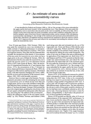
senting the general formulas to analyze a unit square Following Norman (1964), the space in the unit square
with n data points. At the same time, each step will be il- is divided into a region labeled I (for Inferior), since any
lustrated using the 2-point data shown in Figure I, which data point falling in this area represents performance that
follows Norman (1964). The plotted data will be identi- is inferior to that represented by the initial two points. It
fied as (xk,Yk) where the values of k go from I to n, I rep- is the area subtended by the straight lines connecting the
resenting the most confident "yes" response. A rating adjacent data points, including (0,0) and (I, I). That area
scale of n + I points will produce the n points in the unit can be calculated by the trapezoidal rule, Ag, or Brown's
square. The xk values are the proportion of responses R. The general formula for the area I is
with confidence rating k, or lower, made to the new items
(distractors), and the Yk values are the proportion of re- 1= 1/2L(Yk+, + Yk)(xk+1 - xk)
sponses with rating k, or lower, made to the old items L from k = 0 to n. (I)
(targets). The data plotted in Figure I show (x"y,) at
(0.10,0.60) and (x2'Y2) at (0.30,0.80). These data might In the 2-point data of Figure I, the value of I is 0.80.
have come from a recognition task where a person says Thus, we know that the area under an isosensitivity curve
"no" if an item is thought to be new and says either "yes- passing through those two data points has a minimum
value of 0.80. The region labeled S in the upper left rep-
resents superior performance, since any point in that area
represents better performance than do the two initial
l.G0 r----,----::;;;;r--"'T'"-.----..",...
points. Any isosensitivity curve that passes through the
two data points will pass through the three triangles that
remain. They are labeled A, since the exact location of
the isosensitivity curve through those areas is unknown,
.75
and it is ambiguous whether any particular point in those
areas represents superior or inferior performance as
compared with the original data. A'r, the estimate of the
area under the isosensitivity curve, like A', is area I plus
one half of the ambiguous areas. The analysis requires
calculating the slopes and intercepts of the lines in Fig-
ure I and the locations of the interconnecting points
(xk,Yk)'
.15
The first step in the analysis produces the parameters
of the lines that connect and extend beyond adjacent data
points. In the general case, the number of lines always
(xo,Yo).{x· -1 ,y. -1 )
equals the number of points, including (0,0) and (I, I).
.08 ......:..:.::.--=..:.._....L:.-'---'-_---' -'---- --'
Thus, a rating scale with n + I categories generates n data
.00 .Z5 .50 .75 1." points plus the two corners and n + 2 lines. In the ex-
xk
ample, the two points generate four lines. The first line
Figure 1. The unit square containing two data points is shown. (lineo) connects (0,0) to (Xl ,y,) and extends beyond
The data points divide the square into an area below any isosen- (xl>Y,) until it intersects linej. The second line (line.)
sitivity curve that might pass through the two points (Area I), an connects (x, ,y,) to (x2'Y2)' extends below (Xl 'YI) until it
area above any such isosensitivity curve (Area S), and three am-
biguous areas (A). The data (xk,Yd, lines connecting the data intersects the ordinate, and extends above (X2'Y2) until it
points (linek)' and the critical intersections (x"'j"y'l) of those lines intersects the top line where Y equals 1.0. The third line
are shown. See text for further details. (linej ) connects and extends beyond (xbY2) and (I, I),

3. 592 DONALDSON AND GOOD
Table 1
General Format and Worked Example for Calculating A'r
k -I 0 I n n+1 n+Z
xd FA) (0.00) x, xn (1.00)
Yk (H) (0.00) Y, Yn (1.00)
mk (linej ) mo ml mn (0.00)
bk (linej ) (0.00) bl bn (1.00)
x*k (0.00) (0.00) x"j x*n (1.00) ( 1.00)
Yk (0.00) y'O y"j (1.00) (1.00) (1.00)
Area (linej ) Aline., Aline, Aline, Alinen+1
A'r = l/ZI Areatlinej )
A'k A'I A' n
k -I 0 I Z 3 4
xk(FA) (0.00) 0.0 0.30 ( 1.00)
Yk(H) (0.00) 0.60 0.80 ( 1.00)
mk (linej ) 6.0000 1.0000 0.Z857 (0.0000)
bk (Iinej ) (0.0000) 0.5000 0.7143 (1.0000)
xk (0.0000) (0.0000) 0.IZ50 0.5000 ( 1.0000) ( 1.0000)
Yk (0.0000) 0.5000 0.7500 (1.0000) ( 1.0000) ( 1.0000)
Area (Imej ) 0.0469 0.3750 0.7656 0.5000
A'r = 0.8438
A'k 0.8472 0.8348
and the fourth line (linej) connects the point where line , Having established that the slopes of successive lines do
intersects Y = I to (I, I). not increase, row 5 calculates the intercepts (b k) of each
Table 1 shows a format that is useful for doing the re- of the four lines with the ordinate. For line., in any data
quired calculations. The upper part ofthe table is a gen- set, bowill always be 0 and can be entered without calcu-
eral representation showing which values have to be calcu- lation. For line. by Formula 3, b l = YI - (ml)(xI) =
lated and which do not. Entries in brackets, such as (0.00), 0.60 - (1.00)(0.10) = 0.5000. This is the Y value where
require no calculations, and the number, always 0 or 1, line. meets X = 0, the ordinate. For linez, bz = 0.7143, and
can be entered in the table. All other entries require cal- for linej, b3 = 1.0000. The last line, in the general case
culations. The lower part of the table fills in the calcu- line n + 1 and in this case linej, will always have an inter-
lated values for the sample data. The first row, labeled k, cept of I and can be entered without calculation.
identifies the subscripts such as the I in XI and the 2 in The critical points in the calculations become those
Iinej, The next two rows record the actual data. Row 2 points where lines intersect nonadjacent lines. Thus, con-
records the response rates to distractors (xk)' usually sider line. in Figure I. Line. intersects line., at (xI,Yl)
identified as false alarms (FA), and row 3 records the re- and line, at (xz,yz). Those values we know. We need to
sponse rates to targets (Yk)' usually called hits (H). Rows know the intersection point of line. with a line below
4 and 5 are the slopes (mk) and intercepts (b k) of the four (xI'YI)' That point happens to be on the ordinate at a
lines (line., through line-). The general formulas are: point to be called (x~,y~). Similarly, line. intersects the
Y = I line at (x1,Y1)' Line., intersects line, above (xt>YI)
mk = (Yk+ I - Yk)/(xk+ I - xk) (2)
at the point (xt,yt), and its lower intersection is below
bk = Yk - (mk)(xk)' (3) (xo,Yo) at a point labeled (x~ 1,Y~ I)' Since one cannot go
below (xo,Yo), the value of (x~ t>Y~ I) is in fact (0,0) but
These values need to be calculated for each ofthe n + 2
labeling it as conceptually below (xo,Yo) simplifies the
lines except when Table I indicates fixed values. In the
analysis. Similarly, line , goes from (xt,yt) to (x!,yn.
example, there are four lines. Looking at slopes first, by
Line, goes from (X1,Y1) to (x~,y:). Both (x!,yn and
Formula 2, the slope of lineo, mo, is (YI - YO)/(xI - xo) =
(x:,y:) fall beyond (x3'Y3)' but, since that is the limit of
(0.60 - 0.00)/(0.1 0 - 0.00) = 6.0000; the slope ofline I
the unit square, both are in fact at (I, I). Those values can
is ml = (0.80 - 0.60)/(0.30 - 0.10) = 1.0000; the slope
be entered in the table without calculations. Rows 6 and
of line-, m2 = (1.00 - 0.80)/(1.00 - 0.30) = 0.2857; and
7 in Table I present the values of xt and yt, respectively.
the slope of linej, m3 = 0.0000. In any data set of size n,
The general formulas are:
the slope of line n + I will be zero and can be so entered in
the table without calculation. xt = (bk+1 - bk-I)/(mk-I - mk+l) (4)
This first step of calculating the slopes is very impor-
tant since each slope must be less than or equal to the one yt = (mk+l)(xX) + bk+I' (5)
before it. Besides being required for this analysis, the re- By Formula 4, the value for xt
= (0.7143 - 0.00)/
quirement follows Norman's (1964) that the operating (6.00 - 0.2857) = 0.1250 and x1 = (1.00 - 0.50)/
characteristic be monotonic from (0,0) to (I, I) with non- (1.00 - 0.00) = 0.5000. By Formula 5, the value of
increasing slope. In the current example, the slopes go Y~ = (1.00)(0.00) + 0.50 = 0.5000 and yt = (0.2857)
from 6, to I, to less than I, to O. (0.1250) + 0.7143 = 0.7500.

4. Edited by Foxit Reader
Copyright(C) by Foxit Corporation,2005-2009
A'r 593
For Evaluation Only.
Knowing the values of (Xk'Y!> allows the calculation 0.8348. The minimum value with only that one point in
of areas in a variety of different ways. The easiest is to cal- the square is 0.7500 for a range between minimum and
culate the area under each of the four critical lines from maximum of 0.1696. Having two data points rather than
the points where each line intersects the nonadjacent lines. just one cuts the ambiguity almost in half. The amount of
The general formula for the area under line., is: reduction in the ambiguous areas will depend on where
the data points are located in the unit square. Brown (1974)
Aline; = 1/2 (Yk+1 + Y*k-l)(xk+1 - xk-I)' (6)
and Bamber (1975) both point out that the accuracy of
The calculated area under line. goes from (xb,Yb) to the estimates depends on such things as the spacing be-
(x~,y~), and by Formula 6, that area = 1/2(y~ + Y'b) tween data points.
(x~ - Xb) = 1/2(1.0000 + 0.5000)(.5000 - 0.0000) =
0.3750. The important difference between the current DATA
and previous applications of the trapezoidal rule is the use
of the Xk and Yk values rather than the Xk and Yk values. A simple memory experiment was conducted to pro-
The area under each line, is calculated from (Xk-I 'Yk~ I) vide data for a preliminary exploration ofA'r. Twenty uni-
to (Xk+ I ,Yk+ I)' The sum of those areas gives a number versity students were individually tested. Each was given
that includes the I area twice and each of the ambiguous a recognition test on a list of 512 words after having seen
areas once. Dividing that sum by 2 then gives an A'r an initial list of256 words. The test list was organized in
value consisting of area I plus one half of the ambiguous eight blocks of 64 words each, although subjects were
areas. In general, not aware of the blocks. Each block of 64 words included
32 high-frequency and 32 low-frequency words, the sub-
A'r = 1/4 L(Yk+1 + Yk-l)(xk+1 - xk-I)' ject having previously seen half of each. In other words,
L from k = 0 to n + I (7) 16 words of each frequency were old words. The 256
words on the initially presented list were also organized
In the present example the four individual areas are shown
in eight blocks, with 32 words in each block. The first 32
in row 8 labeled Area (linej ). The sum of those values
words presented, 16 high and 1610w frequency, were the
halved is shown in row 9 as A'r. For comparison, Row 10
32 old words in the first test block, albeit in a new ran-
shows the traditional A' values calculated on each of the
dom order from their initial presentation, and randomly
two separate data points. The formula for A' is
mixed with 32 new words, half high and half low fre-
AI. = 0.5 + [(Yk - xk)(I + Yk - xk)]/[4Yk(l - xk)]' quency. Two different presentation lists were used so that
(8) the test words that were new for half the subjects were
old for the other half.
In the limiting case, when one has only one data point, The initial list of words was presented by a computer
that is, n = I, Formula 7 reduces to at the rate of 1.5 sec per word with a 0.5-sec blank inter-
A'r = 0.5 + 1/4(1 + Y'b - X*l)' (9)
val between words. The subjects were instructed simply
to read each of the words out loud and to try to remem-
which in turn reduces to Formula 8. Just as the A' For- ber them. They were told that the list was very long and
mula 8 cannot be used when data points fall below the that they were not to worry when they felt they were not
chance diagonal, so Formula 9 for A'r will yield bizarre
values for below-chance data.
The procedure seems complicated, so perhaps Richard- Table 2
son (1972) was right. But setting up a table such as Table I Sample Raw Data (Subject 85)
on a computer spread sheet and putting the formulas into Confidence Rating
the cells where computations are required makes the 3 Z -I -2 -3
process very simple. The result is a single estimate of the High frequency
area under the isosensitivity curve that uses all the data New 13 16 32 17 31 19
from the rating scale. Like A' itself, the value of A'r can Old 59 23 20 9 12 5
be calculated on individual subject data as long as those Low frequency
New 9 4 8 12 16 79
data satisfy the constraint that the points in the unit square Old 83 5 9 8 12 II
are concave, that is, the successive slopes never increase.
As an example of the extent to which "the addition of Cumulative Data
the second point reduces the ambiguous region in the k=1 k=2 k=3 k=4 k=5
unit square" (Norman, 1964, p. 245), the data in the ex- High frequency
ample yield an A'r of 0.8438. As previously noted, the New 13 29 61 78 109
minimum area from Formula I is 0.80. Thus, the ambig- Old 59 82 102 III 123
uous areas in Figure I have a total area of 0.0876 (twice Low frequency
New 9 13 21 33 49
the difference between A'r and the minimum possible Old 83 88 97 105 117
value). In other words, the area under the isosensitivity Note-s-The entries in each cell are the number of responses (out of
curve is 0.8438 :±: 0.0438. In contrast, had one used only 128) in each rating category to old and new high- and low-frequency
the yes/no data, (xz ,Yz) = (0.30,0.80), the A' value is words. The lower part of the table shows the numbers cumulated.

5. 594 DONALDSON AND GOOD
remembering. The test was given after only a short break The low-frequency data for Subject B5, shown in the
and was self-paced. A 6-point rating scale, ranging from middle of Table 3, were nonmonotonic. The slope de-
-3 (sure new) to +3 (sure old) appeared on the bottom creased from ma through m3 but then increased at m4'
of the screen and remained throughout the test. As each Note that the other calculations are all completed in the
of the 512 words appeared, the subject read it aloud and table but are clearly not meaningful in light of the slope
verbally reported a number representing memory (plus increase. Eliminating the k 4 data point and rerunning the
or minus) and confidence (l, 2, or 3), which was re- calculation produces the satisfactory 4-point solution
corded by the experimenter. After each response, the sub- shown in the bottom of Table 3. Since successive data
ject touched the space bar for the next word to appear. points are cumulative,the k4 data have not been eliminated;
For the initial analyses, each subject's data were orga- instead, they have been collapsed into the k 5 data point.
nized as in Table 2, which shows the data for Subject B5. Each of the 20 subjects provided two data sets, one for
They were then cumulated from the most conservative high- and one for low-frequency words. Of the 40 data
( + 3) category on down, as shown in the lower part of sets, 14 provided complete 5-point estimates ofA'r. Nine-
Table 2. Each set of data was then entered into the gen- teen provided 4-point estimates and 7 had to be reduced
eral formula format of Table 1, with results as shown in to 3-point isosensitivity curves.
Table 3. For Subject B5, the high-frequency data were An obvious question concerns how to transform a
satisfactorily fit on all five data points, as shown by the nonmonotonic 5-point isosensitivity curve to an accept-
consistently declining slopes, mk (Iinej ), The final A'r able 4- or 3-point curve. The first rule would seem to be
value was .7629, as shown. to eliminate any zero entries. Thus, if a person never gave
Table 3
The Analysis of Subject 85's Data in the General Format Shown in Table 1*
High Frequency
k -I 0 I 2 3 4 5 6 7
xk(FA) 0.0000 0.1016 0.2266 0.4766 0.6094 0.8516 1.0000
Yk(H) 0.0000 0.4609 0.6406 0.7969 0.8672 0.9609 1.0000
mk (linej ) 4.5385 1.4375 0.6250 0.5294 0.3871 0.2632 0.0000
bk (Iinej ) 0.0000 0.3149 0.4990 0.5446 0.6313 0.7368 1.0000
xt 0.0000 0.0000 0.1275 0.2529 0.5560 0.7221 0.9525 1.0000 1.0000
yt 0.0000 0.3149 0.5787 0.6785 0.8465 0.9269 1.0000 1.0000 1.0000
Area k 0.0369 0.1256 0.3054 0.3766 0.3660 0.2677 0.0475
A'r 0.7629
A'k 0.7949 0.7954 0.7535 0.7393 0.7127
Ir 0.7494 0.0234 0.0688 0.1797 0.1105 0.2214 0.1455
Low Frequency
k -I 0 I 2 3 4 5 67
xk(FA) 0.0000 0.0703 0.1016 0.1641 0.2578 0.3828 1.0000
Yk(H) 0.0000 0.6484 0.6875 0.7578 0.8203 0.9141 1.0000
mk (linej ) 9.2222 1.2500 1.1250 0.6667 0.7500 0.1392 0.0000
bk (Iinej ) 0.0000 0.5605 0.5732 0.6484 0.6270 0.8608 1.0000
xt 0.0000 0.0000 0.0708 0.1507 0.1432 0.4026 0.4974 1.0000 1.0000
yt 0.0000 0.5605 0.6529 0.7489 0.7344 0.9168 1.0000 1.0000 1.0000
Area k 0.0231 0.0986 0.0502 0.2098 0.3071 0.5726 0.5026
A'r 0.8821
A'k 0.8784 0.8761 0.8734 0.8609 0.8605
Ir 0.8619 0.0228 0.0209 0.0452 0.0740 0.1084 0.5907
Low Frequency (adjusted to 4 points)
k -I 0 I 2 3 4 5 6
xk(FA) 0.0000 0.0703 0.1016 0.1641 0.3828 1.0000
yd H) 0.0000 0.6484 0.6875 0.7578 0.9141 1.0000
mk (linej ) 9.2222 1.2500 1.1250 0.7143 0.1392 0.0000
bk (Iinej ) 0.0000 0.5605 0.5732 0.6406 0.8608 1.0000
xt 0.0000 0.0000 0.0708 0.1495 0.2917 0.5031 1.0000 1.0000
yt 0.0000 0.5605 0.6529 0.7474 0.9014 1.0000 1.0000 1.0000
Area k 0.0231 0.0978 0.1716 0.3090 0.6734 0.4969
A'r 0.8859
A'k 0.8784 0.8761 0.8734 0.8605
Ir 0.8624 0.0228 0.0209 0.0452 0.1829 0.5907
*See text for details.

6. Edited by Foxit Reader
Copyright(C) by Foxit Corporation,2005-2009A'r 595
For Evaluation Only.
a + 3 confidence rating to a new item, the first point on calculations wiU not work because the slope of the line
the isosensitivity curve would be the +2 new-item re- that would connect (xl,YI) with (x2,Y2) is less than that
sponses plotted against the combined + 3 and + 2 old-item from (x2'Y2) to (x3,Y3)' Eliminating (x2,Y2) leaves the data
responses. Four of the 19 4-point estimates were achieved in Figure I. Aaronson suggested that, instead ofthe elim-
by coUapsing unused confidence rating categories. The ination of (x2'Y2), it might perhaps be replaced by some
remaining 15 4-point estimates were obtained as shown point on the line connecting (x"Yl) with (x3'Y3)' The point
in Subject 85's low-frequency data. The increased slope might be one with the same false-alarm rate (x2) and an
(m) at line.,, as compared with linej , points to the col- increased hit rate or perhaps one on the diagonal connect-
lapse of the k 4 data. CoUapsing either of the adjacent ing (x2'Y2) to the upper left-hand corner. In fact, one could
points, either k3 or ks, almost never produced a satisfac- replace (x2,Y2) with any point on the line, and the out-
tory 4-point solution. Thus, the second rule to apply is to come would be the same. First, the minimum area, Ag re-
eliminate the data point at the lower end ofthe line with the mains the same whether (x2,Y2) is eliminated or replaced,
slope increase. FinaUy, of the seven 3-point solutions, two that is, 0.80. Second, no matter what point on the line re-
were obtained by applying both of the above rules. An places (x2'Y2), the resultant A'r value is 0.8375, slightly
unused category was eliminated and then the point at the lower than the value of 0.8438 that is achieved by elim-
lower end of an increasing slope line was eliminated. The inating (x2,Y2)' The latter result obtains because the in-
remaining five 3-point solutions had to correct 5-point clusion of any point on the line forces the isosensitivity
plots that each had two slope increases. In four ofthe five curve to go through the replacement value for (x2'Y2) and
cases, there was a decrease in slope from linea to line" the points on either side. This eliminates the ambiguous
and after that the pattern was increase, decrease, increase, area (A) between (xl,Yl) and (x3'Y3) and above the line
decrease. The final case involved a decrease from linea to connecting them. In other words, any point chosen to re-
line, and from line. to line- and then an increase from place (x2,Y2) forces the curve to assume the lower bound
line- to line, and a further increase from line , to line4' on its path between (Xj,y,) and (x3'Y3)'
That these calculations require that the slopes of suc- Other ways to handle data points that violate the slope
cessive lines be monotonicaUy decreasing is not unusual. restrictions need to be explored. Of those examined, how-
Monotonicity is also a requirement for parametric as- ever, we prefer dropping the offending data point by col-
sessments of isosensitivity curves and is often achieved lapsing it into the one above, because that choice is, in fact,
by using best fitting lines on z-transformed axes. The sug- the most conservative one explored to date. It is so be-
gestion that monotonicity can be achieved in these cal- cause reducing the number of data points on the isosen-
culations by coUapsing the data point at the lower end of sitivity curve increases the size of the ambiguous areas,
a line that increases in slope is only one possibility. Doris leaving a wider possible range about the value of A'r.
Aaronson, in reviewing this paper, suggested an alterna-
tive. Figure 2 shows a fairly typical situation where the DISCUSSION
Is the calculation of A'r worth the effort? For two rea-
1.00 ,.-----r-----,----,.....--....".,. sons, we believe it is. The first concerns the variability of
A'r compared with that of A'. The second concerns the
accuracy of the statistic as an estimate of the area under
the isosensitivity curve.
.75 The question of variability is concerned with the size
of the ambiguous areas (A) surrounding a possible iso-
sensitivity curve. As one reviewer pointed out, however,
the area of ambiguity is related to accuracy of A'r if the
obtained data points faU exactly on the isosensitivity
curve and "sampling variability guarantees that this wiU
not happen." This is, of course, so. But the same situation
exists when one calculates A' or, for that matter, d' from
a single data point. One's data point is simply the best esti-
mate one has.
Consider a single data point (0.2,0.6). The A' value is
0.7917 :::': 0.0917, that is, the ambiguous areas total 0.1834.
•00 e.:-(x~o:.::.y..:=O~)_-l... --l. .L_ .J Suppose that the hit rate (0.6) could actuaUy be any-
.00 .%5 .75 1.00 where between 0.55 and 0.65. A' wiU, of course, be lower
with the former value than with the latter, 0.7685 com-
pared with 0.8137. The lower bound on the lower estimate
Figure 2. The Figure I unit square containing two data points
is shown with the addition ofa third data point (x 2 'Y2) which pro- is 0.6750 and the upper bound on the upper estimate is
duces nonmonotonicity and thus fails to provide a three-point so- 0.9024, for a combined ambiguous area of 0.2274. Con-
lution. sider what happens when one has a second data point,

7. Edited by Foxit Reader
596 DONALDSON AND GOOD Copyright(C) by Foxit Corporation,2005-2009
For Evaluation Only.
(0.4,0.8), on the isosensitivity curve. The two points yield ject comparisons of A' andA'r are less favorable. On high-
A'r = 0.7850 ± 0.0450. Again, suppose that sampling frequency words, A' was as likely to be higher as it was to
variability could put the lower hit rate (0.6) anywhere be- be lower than A'r. Of the 10 cases where A' was lower, 1
tween 0.55 and 0.65 and the higher hit rate between 0.75 was below the lower bound of the individual's A'r value.
and 0.85. If both hit rates were actually at their highest Four of the 10 cases where A' was higher were above the
values, the calcutedA'r = 0.8150 ± 0.0450, and ifboth upper bound on A'r. With low-frequency words, 16 of the
were at the lower end of their range, the calculatedA'r = A' values were below A'r, while only 4 werehigher. Ten of
0.7537 ± 0.0437. The lower bound on the lower estimate the 16 low values were below the lower bound on A'r and
is 0.7100 and the upper bound on the upper estimate is 1 of the 4 higher values was above the upper bound. Thus,
0.8600, for a combined ambiguous area of 0.1500. Even overall, 16 ofthe 40A' values were outside the uncertainty
under the most extreme variability assumptions, the ad- bounds of their respective A'r values. The tendency was
dition ofa second data point reduces the ambiguous areas for A' to underestimate A'r (1 I ofl6) and to be more likely
from 0.2274 to 0.1500. to provide underestimates at higher values of A'r.
One can then compare the area of ambiguity around Finally, perhaps one could more easily handle confi-
A'r as a function of the number of data points one has, dence rating data by calculating the separate A' values
ranging from I (A') on up. As noted in the introduction, for each of the points on the isosensitivity curve and then
as the number of points in the isosensitivity curve in- taking an average. Thus, for Subject B5 's high-frequency
creases, the size ofthe ambiguous areas (A) will decrease. data, one would calculate five separate A' values and av-
And the sample data showed that just moving from one erage them for a final value, which turns out to be 0.7592.
point to two can cut the ambiguity in half. We can now For that person's low-frequency data, one should use
use the present data to further assess the size of that re- only the four points that enter the final A'r calculation
duction in uncertainty. An A' value can be calculated on for comparison with A'r, and that value is 0.8721. This
each person's yes/no data, as can the size of the inferior was done for the 40 data sets, and the comparisons be-
area, I, which represents the minimum possible A' value. tween mean A' and A'r are similar to those between the
Over the 20 subjects, the average A' value on high- yes/no A' and A'r. With high-frequency words, 7 of the
frequency words was 0.7612, and the average minimum mean A' values were lower than A'r and 13 were higher.
value was .6793. The difference between the two is 0.0819, With low-frequency words, mean A' values were lower
so the A' of 0.7612 has a possible range of ±0.0819, or than A'r in 19 of the 20 cases, and II of those 19 were be-
lower and upper bounds of 0.6793 and 0.8431, respec- low the lower bound on A'r. Overall, 18 of the 40 aver-
tively. The average values for the low-frequency words age A' values were outside the range of their comparison
were an A' of 0.8844, an average minimum area of 0.8125, A'r values. Taking an average of multiple A' values is no
and thus A' has a range of ± 0.0719. These can be com- better than simply calculating a single A' on the yes/no
pared with the A'r values from each subject's best isosen- data. And, in either case, almost half of the A' values fell
sitivity curves. For high-frequency words, the average outside the A'r boundaries.
A'r was 0.7597, with a range of ±0.0205, and for low- In conclusion, this paper provides a technique for cal-
frequency words, the A'r was 0.8955, with a range of culating a statistic called A'r. A'r provides an estimate of
±0.0183. A'r has an average range one quarter the size the area under an isosensitivity curve on which one has
of that associated with A' calculated on the yes/no data. any number ofdata points from one on up. The more points
These values are averaged over the 5-, 4-, and 3-point iso- one has on the curve, the less the uncertainty about the
sensitivity curves. Combined over high and low frequency estimate of the area. Numerous writers (e.g., Macmillan
but separately for the 5-, 4-, and 3-point curves, the am- & Creelman, 1991, p. 85) have encouraged researchers
biguous areas were ±0.0145, ±0.0206, and ±0.0257, re- to collect confidence ratings. Until now it has been un-
spectively. Thus, the 3-point fits have almost twice the clear how ratings could be directly integrated into a bet-
ambiguity of the 5-point fits. The average size of the am- ter estimate of the area under the isosensitivity curve. A'r
biguous areas associated with the single-point data (A') is a better measure.
are over five times larger than those with a 5-point solu-
tion, ±0.0769 compared to ±0.0145. REFERENCES
It must be noted that the average A' values for both the
high- and low-frequency words are within the range of AARONSON, D., & WATTS, B. (1987). Extensions of Grier's computa-
tional formulas for A' and s: to below-chance performance. Psy-
uncertainty of their respective A'r values. This suggests
chological Bulletin, 102,439-442.
that, at least for these data, A' is a good estimate ofthe area BAMBER, D. (1975). The area above the ordinal dominance graph and
under the isosensitivity curve, but that becomes a ques- the area below the receiver operating characteristic graph. Journal
tion of accuracy to which we now turn. ofMathematical Psychology, 12,387-415.
A'r is simply a better estimate of the area under the iso- BROWN, J. (1974). Recognition assessed by rating and ranking. British
Journal ofPsychology, 65, 13-22.
sensitivity curve than is A'. The comparison above of the BROWN, J. (1976). An analysis ofrecognition and recall and of prob-
average A'r to the average A' values obtained from the lems in their comparison. In 1. Brown (Ed.), Recall and recognition
yes/no data was not unfavorable. However, subject by sub- (pp. 1-36). London: Wiley.

8. A'r 597
DONALDSON, W. (1992). Measuring recognition memory. Journal of POLLACK, I., & NORMAN, D. A. (1964). A non-parametric analysis of
Experimental Psychology: General, 121,275-277. recognition experiments. Psychonomic Science, 1,125-126.
DONALDSON, W. (1993). Accuracy of d' and A' as estimates of sensi- POLLACK, I., NORMAN, D. A., & GALANTER, E. (1964). An efficient
tivity. Bulletin ofthe Psychonomic Society, 31, 271-274. non-parametric analysis of recognition memory. Psychonomic Sci-
GREEN, D. M. (1964). General prediction relating yes-no and forced- ence, 1,327-328.
choice results. Acoustical Society ofAmerica, 36, 1042. RICHARDSON, J. T. E. (1972). Nonparametric indexes of sensitivity and
GREEN, D. M., & MOSES, F. L. (1966). On the equivalence of two recog- response bias. Psychological Bulletin, 78,429-432.
nition measures of short-term memory. Psychological Bulletin, 66, SIMPSON, A. J., & FITTER, M. J. (1973). What is the best index of de-
228-234. tectability? Psychological Bulletin, 80, 481-488.
GRIER, J. B. (1971). Nonparametric indexes for sensitivity and bias: SNODGRASS, J. G., & CORWIN, J. (1988). Pragmatics of measuring
Computing formulas. Psychological Bulletin, 75, 424-429. recognition memory: Applications to dementia and amnesia. Jour-
MACMILLAN, N. A., & CREELMAN, C. D. (1991). Detection theory: A nal of Experimental Psychology: General, 117, 34-50.
user s guide. Cambridge: Cambridge University Press.
NORMAN, D. A. (1964). A comparison of data obtained with different
false-alarm rates. Psychological Review, 71, 243-246.
POLLACK, I., & HSIEH, R. (1969). Sampling variability of the area (Manuscript received August II, 1995;
under the ROC-curve and of d:. Psychological Bulletin, 71, 161-173. revision accepted for publication January 23, 1996.)