This is one of two exams given to our students this year. They had two hours to solve three problems and had to return R codes as well as handwritten explanations.

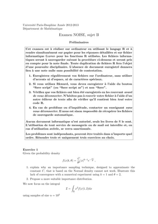
1. Universit´ Paris-Dauphine Ann´e 2012-2013
e e
D´partement de Math´matique
e e
Examen NOISE, sujet B
Pr´liminaires
e
Cet examen est ` r´aliser sur ordinateur en utilisant le langage R et `
a e a
rendre simultan´ment sur papier pour les r´ponses d´taill´es et sur fichier
e e e e
informatique Examen pour les fonctions R utilis´es. Les fichiers informa-
e
tiques seront ` sauvegarder suivant la proc´dure ci-dessous et seront pris
a e
en compte pour la note finale. Toute duplication de fichiers R fera l’objet
d’une poursuite disciplinaire. L’absence de document enregistr´ donnera
e
lieu ` une note nulle sans possibilit´ de contestation.
a e
1. Enregistrez r´guli`rement vos fichiers sur l’ordinateur, sans utiliser
e e
d’accents ni d’espace, ni de caract`res sp´ciaux.
e e
2. Si vous utilisez Rkward, vous devez enregistrer ` l’aide du bouton
a
“Save script” (ou “Save script as”) et non “Save”.
3. V´rifiez que vos fichiers ont bien ´t´ enregistr´s en les rouvrant avant
e e e e
de vous d´connecter. N’h´sitez pas ` rouvrir votre fichier ` l’aide d’un
e e a a
autre ´diteur de texte afin de v´rifier qu’il contient bien tout votre
e e
code R.
4. En cas de probl`me ou d’inqui´tude, contacter un enseignant sans
e e
vous d´connecter. Il nous est sinon impossible de r´cup´rer les fichiers
e e e
de sauvegarde automatique.
Aucun document informatique n’est autoris´, seuls les livres de R le sont.
e
L’utilisation de tout service de messagerie ou de mail est interdite et, en
cas d’utilisation av´r´e, se verra sanctionn´e.
e e e
Les probl`mes sont ind´pendants, peuvent ˆtre trait´s dans n’importe quel
e e e e
ordre. R´soudre trois et uniquement trois exercices au choix.
e
Exercice 1
Given the probability density
C k−1 − |x|
f (x|k, θ) = |x| e θ ,
θk
1. explain why an importance sampling technique, designed to approximate the
constant C, that is based on the Normal density cannot not work. Illustrate this
lack of convergence with a numerical experiment using k = 1 and θ = 2.
2. Propose a more suitable importance distribution.
We now focus on the integral
I= x2 f (x|1, 2)dx
R
using samples of size n = 102

2. 3. Propose a Monte Carlo approximation of I. (Hint : Note that the integral over R
is twice the integral over R+ and connect f with a standard distribution on R+ .)
4. Approximate I by importance sampling using the same distribution g as in question
2.
5. Compute a confidence interval on I at level 95% for each of your method. Which
one of the two estimates does reach the lowest precision ?
6. Design a Monte Carlo experiment in order to check whether or not the asymptotic
coverage level of the CI holds. Repeat the experiment with samples of size n = 103 .
Exercice 2
Given the density on R∗ ,
+
β α −α−1 − β
f (x|α, β) = x e x
Γ(α)
1. Determine which of the following distributions can be used in an A/R algorithm
designed to sample from f (x|2, 4) :
k x k−1 −(xλ)k 1 1 k−1 − x
g1 (x) = ( ) e g2 (x) = x e θ g3 (x) = (1 + αx)−1/α−1
λ λ θk Γ(k)
which are respectively a Weibull, a Gamma and a generalized Pareto distribution
density. (Motivate your choice.)
2. Using the inversion method write an algorithm that samples from the selected g.
3. Write an R function AR() that samples from f (x|2, 4). (Extra-credit : Optimize the
parameters of the proposal density g.)
4. Based on a sample of size 104 from f (x|2, 4), estimate by Monte Carlo the mean
and variance of h(X) = 1/X and give a confidence interval at level 95% for both
quantities.
5. The distribution associated with f can be obtained by the transform 1/Z where
Z ∼ Gamma(α, 1/β). Establish this result and test it, based on the sample used in
question 4.
Exercice 3
If X1 , X2 , . . . , Xk is a sample from the N (0, 1) distribution, then Yk = Xi2 follows the
χ 2 (k) distribution. We wish to verify a convergence theorem due to R. A. Fisher which
states that √ L
2Yk − 2k − 1 − − N (0, 1)
−→
k→∞
1. Create a function rchisq2(n,k) which simulates n realizations of the χ2 (k) distri-
bution, using nk realizations of the standard normal distribution. (Note : if you do
not manage this question, you can use the R function rchisq() for the remainder
of the exercise.)
√ √
2. For k = 50 and n = 1000, propose a graphical way to verify the fit of 2Yk − 2k − 1
to the N (0, 1) distribution.
3. Using ks.test() and n = 1000, check whether the normal distribution is an accep-
table fit when k = 3, k = 30, k = 300.

3. 4. From now on, k = 300 and n = 1000. We now have a test to check the fit of a
sample x to the χ2 (k) distribution : we accept the null hypothesis that x comes
from √ χ2 (k) distribution iff the Kolmogorov-Smirnov test accepts the hypothesis
the √
that 2Yk − 2k − 1 fits the N (0, 1) distribution. Perform a bootstrap experiment
to calculate the probability of accepting the null hypothesis for a sample which
comes from the Beta(1, k) distribution.
5. Perform another bootstrap experiment to calculate the same probability when using
directly the Kolmogorov-Smirnov test for fit to the χ2 (k) distribution (whose cdf
exists in R as pchisq).
Exercice 4
The F rechet(α, s, m) distribution defines a random variable X which takes values in
]m, +∞[ and with cumulative distribution function
−α
x−m
F (x) = exp −
s
1. Using the generic inversion method, write a function rfrechet(n,α,s,m) which
outputs n realizations of the F rechet(α, s, m) distribution.
2. For α = 5, s = 1, m = −3, give a Monte Carlo experiment to estimate V ar(X)
and the median of X. Calculate (on paper) the theoretical value of the median and
compare it to your estimate.
3. Propose a bootstrap experiment to evaluate the bias of your variance and median
estimators.
4. For α = 5, s = 1, m = −3, use the Kolmogorov-Smirnov test to verify that the
variable α
1
Y =
X −m
follows an Exp(1) distribution.
Exercice 5
Consider the density function on the real line R
(2k + 1)! Φ(x)k Φ(−x)k
fk (x) = √
(k!)2 2π exp(x2 /2)
where k ≥ 1 is an integer and Φ is the normal cdf.
1. Check by numerical integration that fk is a proper density for k = 6, 12, 24
2. Design an accept-reject algorithm function on R that produce an iid sample of
arbitrary size m for an arbitrary parameter k. (Hint : Notice that either Φ(x)
or Φ(−x) is necessarily less than 1/2 and that Φ(−x) = 1 − Φ(x). Deduce that
Φ(x)Φ(−x) < 1/4.) Produce a graphical verification of the fit for m = 103 and
k = 6, 12, 24.
3. We want to check from the acceptance rate of this accept-reject algorithm that
the normalisation is correct in the above. Produce 250 realisations of an empirical
acceptance rate based on 100 proposals and deduce a 97% confidence interval on
the expectation of the acceptance rate. Check whether or not it contains the inverse
normalising constant.

4. 4. This density is actually the distribution of the median of a normal sample of size
n = 2k + 1. (Extra-credit : Establish this rigorously.) Generate a sample from the
above accept-reject algorithm with m = 250 and k = 10, then another sample of
m = 250 medians from samples of 21 normal variates. Test whether they have the
same distribution.
5. Check whether or not the p-value of the above test is distributed as a uniform U (0, 1)
random variate.
Exercice 6
Download the dataset Nile :
> data(Nile)
> nile = jitter(as.vector(Nile))
We will assume that those are iid realisations of a random variable X, producing a
sample Xn = (X1 , . . . , Xn ).
We denote by IQ0.8 (Xn ) an inter-quantile interval of the sample, defined by
IQ0.8 (Xn ) = Q0.9 (Xn ) − Q0.1 (Xn )
where Q0.9 (Xn ) and Q0.1 (Xn ) are the empirical quantiles of the sample at levels 90%
and 10%. We would like to calibrate IQ0.8 (Xn ) by a coefficient α so that it becomes an
unbiased estimator of the standard deviation of the distribution of the Xi ’s.
1. Write an R function iqan(x) which produces the statistic IQ2 (Xn ) associated
0.8
with the sample x. Compute the outcome of your function on the dataset nile.
2. Simulate 104 replicas of a Cauchy C(µ, σ) (µ being the location and σ the scale)
sample Xn of size n = 100 and deduce a Monte Carlo evaluation of the coefficient
α such that αE[IQ2 (Xn )] = σ 2 . (Extra-credit : Explain why the values of µ and σ
0.8
can be chosen arbitrarily.)
3. Based on the previous experiment, and using the 104 realisations of IQ0.8 (Xn )
generated in question 2., deduce a 93% confidence interval on IQ0.8 (Xn )/σ. (Hint :
Use the empirical cdf, rather than bootstrap.) Compare with the asymptotically
normal 93% confidence interval on E[IQ0.8 (Xn )]/σ. Check whether or not 6.1554
belongs to these intervals. (Extra-credit : Justify the choice α = 1/6.1554.)
4. By running a Monte Carlo experiment based on 105 replications of Cauchy random
variates with location µ and scale σ of your choice, check whether or not the 93%
confidence interval on log |X − µ| contains log(σ).
We will assume in the rest of the exercise that µ = Q0.5 (Xn ), the median of the sample,
˜
and
σ (Xn ) = exp{(log |X1 − Q0.5 (Xn )| + . . . + log |Xn − Q0.5 (Xn )|)/n}
˜
are acceptable estimators of µ and σ. (Extra-credit : Explain why the usual empirical
moments do not work for the Cauchy distribution.)
5. Check whether or not nile is distributed from a Cauchy sample (with unknown
location and scake).
6. Since nile is not necessarily a Cauchy sample, denoting by σ the standard deviation
of the distribution of the Xi ’s, construct by bootstrap a 93% confidence interval on
IQ0.8 (Xn )/σ, using σ (Xn ) based on nile as the estimate of σ. Does it still contain
˜
6.1554 ?