Economic Feasibility of Shale Gas

MARIO KHATER
ASSESSING THE ECONOMIC FEASIBILITY OF SHALE GAS
A North American Perspective
An Economic Insight into Production Decline Curve Analysis
Mémoire présenté
à la Faculté des études supérieures et postdoctorales de l’Université Laval
dans le cadre du programme de maîtrise en économique
pour l’obtention du grade de Maître ès arts (M.A.)
DÉPARTEMENT D’ÉCONOMIQUE
FACULTÉ DES SCIENCES SOCIALES
UNIVERSITÉ LAVAL
QUÉBEC
2013
© Mario Khater, 2013

ii
Résumé
Ce mémoire étudie la faisabilité économique de la production de gaz de shale à partir de cinq
formations géologiques différentes (le Marcellus, le Barnett, le Haynesville, le Montney et
l’Utica) dispersées aux États-Unis et au Canada. Depuis 1990, le progrès technologique,
notamment en termes de forage horizontal et de fracturation hydraulique, a permis la
production économique du gaz naturel à partir de shales et a amélioré les perspectives à long
terme pour l’approvisionnement en gaz naturel en Amérique du Nord. L'Energy Information
Administration (EIA) prévoit que d'ici 2046 près de 50% de l'approvisionnement en gaz naturel
américain proviendra du gaz de shale; d'autres chercheurs estiment que l'approvisionnement
en gaz naturel en Amérique du Nord, sous forme de gaz de shale, durera plus de 100 ans. Ainsi,
ce gaz non conventionnel est censé révolutionner les perspectives futures du développement
énergétique. Cependant, une fois exploité, sa mise en valeur reste incertaine vue que sa
rentabilité économique est vulnérable et dépend de plusieurs facteurs économiques et
géologiques. Notre projet déterminera l’état général de la production de la ressource via
l’interprétation des courbes de déclin et l’analyse des économies de seuils de rentabilité et aura
deux volets: (1) technique et (2) économique. Premièrement, dans la partie technique, on
analyse les courbes de déclin afin de prédire comment est ce que les réserves de gaz de shale
sont estimées dans l'industrie. Deuxièmement, dans la partie économique, qui, par l'évaluation
des tendances à la baisse de la production de gaz de shale, nous permettra d’identifier les
divers agrégats qui rendent cette production, économiquement rentable. En conclusion, on
développe un modèle logistique de déploiement des puits pour le shale d'Utica illustrant
l'impact potentiel des volumes de gaz produits, le temps de déploiement des puits, le nombre
de puits forés, ainsi que des redevances versées sur la rentabilité économique du projet.

iii
Abstract
This thesis analyzes the economic feasibility of producing shale gas from five different shale
formations (Marcellus, Barnett, Haynesville, Montney, and Utica) dispersed in the United States
(U.S.) and Canada. Since 1990, advances in technology, mainly horizontal drilling and hydraulic
fracturing have allowed economic production of natural gas from shales and boosted the long-
term outlook for the supply of natural gas in North America. The Energy Information
Administration predicts that by 2046 almost 50% of the U.S. natural gas supply will come from
shale gas; other researchers estimate that the natural gas supply in North America, in the form
of shale gas, will last more than 100 years. Thus, shale gas is thought to be the game changer of
the course of future energy development trends; however, its economic profitability is
vulnerable and depends upon several economic and technical factors. Our study is conducted
through Decline Curve Analysis and breakeven economics and has two facets: (1) technical and
(2) economic. First, the technical part consists on investigating Production Decline Curve
Analysis in order to understand how shale gas reserves are estimated in the industry. Second,
comes the economic part, which by assessing steep initial decline trends of gas production from
five major shale plays, focuses on identifying both geologic and economic aggregates that
render shale gas production, economically profitable. Finally, to better understand the
economic functionality of producing shale gas, we develop a logistic growth model of wells
deployment for the Utica shale that depicts the potential impact of volumes of gas produced,
wells deployment time, number of wells drilled, and royalties paid on the project economics.

iv
Acknowledgments
I would like to thank many persons who contributed to the accomplishment of my master
degree project.
First of all, I would like to express my gratitude to my supervisor, Pr Patrick González. I am
thankful for your valuable insights and directions that gave me needful guidance to complete
the research and write my thesis. I also thank you for being there during my entire project. I
thank you for your patience and persistence with the help and assistance that you offered me. I
also thank you because you made the most difficult tasks so easy to accomplish and to
understand.
I would also like to thank my friend Rana Daher for all the support, help and encouragement
she gave me.
Finally, I thank my beloved family who supported me during all my life; I would not be able to
succeed without you. I thank you for believing in me. I thank you for the love and care you gave
me. I thank my mother Norma for all the efforts she made for me. I thank you for being there
for me and with me at all times despite the great distances that separated us. I also thank my
father Elia for the trust and the guts you built in me and the great generosity and modesty that I
carved through you. I thank my three brothers Georges, Rami and Hicham for their love and
support. Finally, to my cousin Ziad, I thank you for the infinite generosity, the kindness and the
gracious hospitality that you extended to me during my entire stay at your place.

“Natural gas is the best transportation fuel. It's
better than gasoline or diesel. It's cleaner, it's
cheaper, and it's domestic. Natural gas is 97%
domestic fuel, North America. ”
𝑇ℎ𝑜𝑚𝑎𝑠 𝐵. 𝑃𝑖𝑐𝑘𝑒𝑛𝑠 (1928−)
“Natural gas is the future. It is here.”
𝐵𝑖𝑙𝑙 𝑅𝑖𝑐ℎ𝑎𝑟𝑑𝑠𝑜𝑛 (1947−)
𝑇𝑜 𝑚𝑦 𝑏𝑒𝑙𝑜𝑣𝑒𝑑 𝑓𝑎𝑚𝑖𝑙𝑦,

VI
Table of contents
Résumé ........................................................................................................................................... II
Abstract.......................................................................................................................................... III
Acknowledgments.......................................................................................................................... IV
List of Figures ............................................................................................................................... VIII
List of Tables .................................................................................................................................. IX
Abbreviations.................................................................................................................................. X
Table of conversion......................................................................................................................... X
Introduction .................................................................................................................................. 11
Literature Review.......................................................................................................................... 13
Chapter I: Shale Gas and Production Decline Curve Analysis...................................................... 14
1.1. Definition: What is Shale Gas? ......................................................................................... 14
1.2. How Shale Gas is produced? ............................................................................................ 15
1.2.1. Horizontal Drilling ............................................................................................................ 15
1.2.2. Hydraulic Fracturing......................................................................................................... 16
1.3. Understanding Production Decline Curve Analysis.......................................................... 17
1.3.1. History of Reserves Estimates Calculation Methods ....................................................... 17
1.3.2. PDCA in unconventional reservoirs.................................................................................. 20
1.3.2.1. Exponential truncation of hyperbolic equations............................................................. 21
1.3.2.2. Multiple transient hyperbolic exponents ........................................................................ 21
Chapter II - The economics of shale gas wells .............................................................................. 23
2.1. Model, Methodology, Variables....................................................................................... 25
2.1.1. Cash flow analysis ............................................................................................................ 25
2.1.1.1. Explaining the model variables........................................................................................ 25
2.1.2. Sensitivity analysis............................................................................................................ 27
2.1.3. Decision making parameters............................................................................................ 28
2.1.3.1. Net Present Value............................................................................................................ 28
2.1.3.2. Internal Rate of Return (IRR) ........................................................................................... 29
2.1.3.3. Payout Period................................................................................................................... 30

VII
2.2. Shale plays and model assumptions:............................................................................... 30
2.2.1. Barnett.............................................................................................................................. 31
2.2.2. Marcellus.......................................................................................................................... 35
2.2.3. Haynesville ....................................................................................................................... 37
2.2.4. Montney........................................................................................................................... 39
2.2.5. Utica ................................................................................................................................. 41
2.3. Economic discussion......................................................................................................... 42
2.4. A logistic distribution model of wells deployment (Utica Shale) ..................................... 46
2.4.1. Model and Assumptions .................................................................................................. 47
2.4.2. Economic discussion ........................................................................................................ 50
Conclusion..................................................................................................................................... 54
Appendix ....................................................................................................................................... 55
References .................................................................................................................................... 88

VIII
List of Figures
Figure 1: Conventional, tight, and shale gas and oil. ................................................................................ 14
Figure 2: Stages of a shale gas production process. ................................................................................. 16
Figure 3: DCA, rate versus cumulative gas production. ............................................................................ 21
Figure 4: Energy trends in the U.S............................................................................................................. 23
Figure 5: Natural gas production by source, 1990-2030 (tcf) ................................................................... 23
Figure 6: Shale Gas Production Economics (Banks 2008) ......................................................................... 24
Figure 7: Comparison of number of wells drilled (per year)..................................................................... 46
Figure 8: Truncation of hyperbolic equations........................................................................................... 56
Figure 9: Arps Type curves ........................................................................................................................ 56

IX
List of Tables
Tables 1, 2 (a, b, c, d, and e): Shale plays models parameters and expected ranges...........................31-41
Table 3: Sensitivity Analysis Results...........................................................................................................43
Table 4: Estimating gas reserves using Arps equations .............................................................................58
Table 5: Quebec’s New Royalty Regime (NRR) ..........................................................................................61

X
Abbreviations
bcf billion cubic feet
EIA Energy Information Administration
EUR Estimated Ultimate Recovery
FYP First Year Price
GP Gas Produced
IRR Initial Rate of Return
md Millidarcy
Mmcf Million cubic feet
NPV Net Present Value
OGIP Original Gas in Place
PDCA Production Decline Curve Analysis
RF Recovery Factor
TRR Technically Recoverable Resources
mcf Thousand cubic feet
tcf trillion cubic feet
U. S. United States
Table of conversion
tcf bcf Mmcf mcf
1 tcf 1 1,000 1,000,000 1,000,000,000
1 bcf 0,001 1 1,000 1,000,000
1 Mmcf 0.000001 0.001 1 1,000
1 mcf 0.000000001 0.000001 0.001 1

11
Introduction
Shale gas reservoirs differ from conventional gas reservoirs in the fact that it is the process of making a
well ready for production that forms the reservoir (T.A. Blasingame 2008). Since their permeability is
very low, a multi-stage conductive platform is required between the well completion and the reservoir
to attain commercial economic rates. To achieve the latter, massive multi-stage hydraulic fracture
techniques are used to boost the interconnectivity between the fractures of the well (Gaskari R. and
Mohaghegh 2006). The linkage and spacing of the induced fracture networks are still generally not very
well understood. Therefore producing companies are grandly motivated to enhance their understanding
of these characteristics and this for two reasons: (1) to get more reliable and accurate production and
reserve estimates, and (2) to ameliorate their interpretation of the available data in order to enhance
their field development strategies and drill, economically, more fruitful wells (M. Y. Soliman, Johan Daal
and al. 2012).
In general, shale gas plays present various challenges to analysis that conventional reservoirs simply do
not imply. Their very low permeability makes conventional production almost impossible; thus every
well in a shale play must be hydraulically fractured to achieve economical production (Holditch S. A.
2006; Sunjay 2012).
As for the techniques applied to estimate potential recoverable reserves contained in underground
shale reservoirs, Production Decline Curve Analysis (PDCA) was seen as the most successful
characterization technique because it is practical, reliable, and relatively costless (Poston 2005). PDCA is
a traditional graphical procedure that monitors and predicts gas production decline rates over time. It is
relatively costless because, once compared to other characterization techniques, (1) it is mainly based
on extrapolation techniques (a simple assessment of past performance production data of pre-
established wells), and so (2) previous production decline trends will be projected in order to predict
future potential behavior of newly discovered wells.
Among various methods that can be used within the industry to estimate Gas In Place1
(GIP) in a
particular shale formation, those advanced by Arps (1945) and Fetkovich (1987) are thought to be the
most popular ones2
. They were originally designed to forecast and predict production capacities of
conventional reservoirs and vertical wells but once applied solely to the estimation of unconventional
gas reservoirs they encounter major key issues and provide unreliable results (Lisa Dean P. Geol. and Eng
2008). Since 2006, shale gas reservoirs started to be widely explored and developed in North America,
notably in the U.S., with advances in technology, such as multi-fractured horizontal wells and directional
drilling, being the key drivers for success.
1
The estimated gross quantity of gas contained within every shale gas play or reservoir.
2
The first successful horizontal drilling act that contributed the most to the launching of the North American Shale Gas
Revolution was driven by a small private company, Mitchell Energy; it took place in the North Texas Barnett Shale region,
and it dates from 1991 (Wikipedia).

12
Nowadays, shale plays that have been exploited had numerous and complex reservoir and production
characteristics that rendered the mathematical estimation of gas produced from horizontal wells
deceptive because it often leaded to unreasonable production estimates (Fekete associates Inc. 2004).
The characterization process of shale plays in terms of future production capabilities is divided into two
basic elements: (1) the evaluation of the reservoir technical properties (permeability, GIP, etc.) and, (2)
the prediction of future production trends of newly discovered wells, being a crucial part of the
characterization process, enabling producing companies to estimate existing volumes of Technically
Recoverable Resources3
(TRR) in shale plays and eventually to assess the economic profitability of every
well drilled (within that play). To this end, this project proposes a base case economic model that
facilitates the tasks of evaluating and assessing the profitability of shale gas investments.
Essentially, the assessment of shale plays economics goes through two key stages: the technical
(estimating gas reserves) and the economic (William M. Gray, Troy A. Hoefer and al. 2007). From this
perspective, our study combines theory modeling and empirical testing in an application field that is
novel to the energy economics literature.
The first chapter of our project is entitled: “Shale Gas and Production Decline Curve Analysis”. At first, it
will be question to present a brief literature review of the economics of extracting natural gas from
shale followed by an attempt to advance answers to three basic questions: (1) What is shale gas? (2)
How shale gas is produced? (3) How shale gas reserves are estimated by operators using PDCA?
Later on, comes the second chapter of our project, through which, by analyzing various production
decline scenarios of some major shale plays in the U.S. and Canada (Marcellus, Haynesville, Barnett,
Montney, and Utica), we identify the economic thresholds that will render shale gas projects
economically productive and will hence allow us to detect the economic parameters that impact the
productivity of a shale gas reservoir. Our second chapter is entitled “The Economics of Shale Gas Wells”.
The latter offers a microeconomic insight into PDCA and the analysis is done following a 2-step
methodology: (1) Cash flow analysis (to assess the economic feasibility of the project), and (2) Sensitivity
analysis (to monitor how the economics of the project will vary under various cost-production
development scenarios). To note that the results found will be stated in terms of NPV (Net Present
Value), IRR (Internal Rate of Return) and Payout Periods.
Additionally, since the Utica shale is still in its early stages of development, a simple logistic model that
describes the relationship between volumes of gas produced, royalties, and wells deployment time on
the scale of the industry will also be proposed. The latter will depict how annual royalties collected (by
the government) are positively correlated with continuous drilling activities and how these royalties will
tend to dramatically fall post-deployment time.
3
The volume of gas which is recoverable using available exploitation and production technology without regard to cost,
which is a fraction of the estimated GIP.

13
Literature Review
How gas reserves are estimated from unconventional reservoirs plays a central role in assessing the
economic feasibility of shale plays (Larry Lake, John Martin and al. 2012). Five years ago, an increasing
number of authors, with or without academic affiliations, started to investigate and to evaluate the
economic profitability of shale plays (Andrew Potter, Helen Chan and al. 2008; Al-Reshedan 2009; Jeff
Ventura, Aubrey k. McClendon and al. 2009; Bailey 2010; Kaiser 2010; Lin 2010; Jason Baihly, Raphael
Altman and al. 2011; Kaiser 2012; Larry Lake, John Martin and al. 2012; Mason 2012). However, the
assessment of shale plays economics is volatile and the calculated results depend upon the reliability of
the assumptions made (in terms of gas price, drilling and completion costs, etc.) before the launch of the
analysis. Whilst some assumptions are common to all shale plays, some others are specific to every
shale play. The latter varies based on several criteria’s, such as: geographical locations, reservoirs
physical properties, proximities to market hubs, etc. In our project, we outline, for every shale play, a
specific set of assumptions (Chapter II) and we make a logical interference into the existing literature on
shale gas economics by proposing a flexible economic model that fits all types of shale plays.
Part of the theory developed in this project relies on financial analysis formulas that appraise the
impacts of the model input-parameters (economic and geologic) variations on the expected financial
outputs of the investment. This methodology has been used, among others, by Lin (2010), Bailey (2010),
and Kaiser (2012) to test the economics of the Utica, the Barnett and the Hayneville plays, respectively.
The typical focus of this literature is to test the economic feasibility of every shale play under different
development and market scenarios. In contrast, our study uses cash flow sensitivity analysis to forecast
the total stream of financial earnings that could derive from the development of every shale play as well
as to study how these anticipated financial outcomes could, over time, increase or decrease based on
prevailing economic conditions. Moreover, we introduce a logistic growth model that assesses the
impact of wells deployment on both volumes of gas produced and annual royalties paid within the
industry in the Utica shale.
Finally, the evaluation of the economic profitability of shale plays is related to a stream of technical work
that deals with the estimation of future gas reserves from unconventional formations (Lisa Dean P. Geol.
and Eng 2008; Liu Wendy 2008; Jason Baihly, Raphael Altman and al. 2011). The existing literature on
shale gas economics is limited in a several number of ways. Mainly, it has not evaluated the economic
profitability of producing shale gas while taking into account the fact that it is of a central importance to
understand how volumes of gas, that will be in later years, produced and sold, are estimated in the first
place, nor has it presented a clear economic explanation of the methods and technical variables that are
used within the industry to estimate gas reserves from unconventional formations.

14
Chapter I: Shale Gas and Production Decline Curve Analysis
Normally, shale gas plays contain both free (contained within the natural fractures of shale) and
adsorbed gas (accumulated on a solid material such as the organic particles in a shale reservoir)4
. The
latter is rarely commercially produced however the former is the major contributor to economic
production. Gas production from shale gas wells is often estimated using traditional decline curves
(PDCA) developed by Arps in 1945 and is mainly characterized by high initial production rates, steep
decline rates and long term steady low production rates, thereafter.
1.1. Definition: What is Shale Gas?
Shale gas is natural gas trapped in an organic-rich, fine-grained underground rock called shale (González
2012). Shale gas is found in shale formations. It is produced from the fractures and micropores spaces of
shales. By shales we mean those underground sedimentary rocks composed of clay and fragments of
other minerals such as quartz and calcite (SCGNC 2006). Shale gas is normally generated during
underground burial, when heat and pressure crack the organic accumulations. During the process of
generation, some of the oil-gas, with high permeability, succeeds to flow and migrate to less deep
wellbores (relatively close to the surface), forming the so-called conventional reservoirs, while some
other, shale gas (with low permeability), for example, do not succeed to escape the organic matter and
still trapped within the shale formation. The latter is the so-called unconventional reservoirs (Holditch S.
A. 2006).
Figure 1: Conventional, tight, and shale gas and oil. Adapted from EIA (2011) and Kaiser (2012).
Hence, given that typical shale reservoirs are buried few kilometers deep in the ground and are largely
distributed over extensive geographic zones rather than concentrated in specific locations, gas shales
are usually known as resource plays or reservoirs (Larry Lake, John Martin and al. 2012).
4
Source: Schlumberger Oilfield Glossary.
Land_surface
Conventional_non_associated_gas Coalbed_methane
Conventional_associated_gas
Seal
Conventional_oil
Sandstone
Tight_sand_gas
Tight_sand_oil
Oil-rich_shale Gas-rich_shale
Drilling_rigs

15
The NEB Report (2009) states that the volume of natural gas, contained within every shale play depends
of the thickness and geographic extent of the reservoir. Thus, volumes of GIP increase -the thicker is the
reservoir- as the geographic extent of the reservoir grows.
Finally, low permeability indicates the restricted capacity for shale gas to flow easily through shale
formations, the reason why, usually, unconventional reservoirs development require more complex
stimulation techniques to be economically produced than is the case with conventional reservoirs (T.A.
Blasingame 2008).
1.2. How Shale Gas is produced?
As noted earlier, shale gas will not easily migrate to any vertical well drilled through it because of the
low permeability of shales. Fortunately, recent advances in technology succeeded to solve this problem
(Jason Baihly, Raphael Altman and al. 2011). Every decision concerning the eventual commercial
development of shale gas requires, ex ante, several years of exploration, collection of data and trials.
The different stages that are linked to the exploration activities require the existence of an entity (e.g.
producing firm) that is ready (financially capable) to offer whatever huge, but necessary funding without
having any guarantee that the project will finally succeed (KPMG Global Energy Institute 2011).
Every entity proceeds to the development of shale gas according to its own methodologies and beliefs
but, in general, the process goes through five different stages of exploration and evaluation before it
comes to the stage of commercial development. Each one of these stages consists in collecting technical
information that, once analyzed and executed, will enable the producing firm to pass to the next stage
of the producing process. Since the majority of unconventional oil-gas plays are seen to be of low
permeability, their production process, once taking place, will require the adoption of specific methods
to increase the surface of the reservoir, in liaison with the well. As already pointed, two methods are
being currently used: (1) horizontal drilling, and (2) (multi-stage) hydraulic fracturing (fracking).
1.2.1. Horizontal Drilling
Firstly, the drilling has to be vertical. The depth of the vertical well is proportional to the depth of the
underground location of the shale formation. The former has to stay above the latter. The issue of -low
permeability gas production- being uneconomic is now offset by drilling horizontal wells, where the drill
bit (cutting tool) is directed from its free fall trajectory to follow a more horizontal path (upon an
increasing curvature) for one to two kilometers (can go to 2.5 km), thereby connecting the wellbore to
as much reservoir as possible (SCGNC 2006; M. Y. Soliman, Johan Daal and al. 2012).
The horizontal drilling enhances the likelihood of the wellbore to intersect with a much great number of
naturally existing fractures in the reservoir. The trajectory of the drill path changes with the changing of
the fracture trends in every zone. The arbitration between drilling horizontally or vertically is enhanced
access to the reservoir (increases the possibility of recovering more gas); however this is surely done at a
way larger cost. Lee (2011) points that drilling is challenging since drilling costs typically comprise half of

16
the cost of the wells and access to the reservoir is improved with horizontal drilling which may access a
longer productive zone within the reservoir than vertical wells, which the author qualifies as cheap.
1.2.2. Hydraulic Fracturing
Hydraulic fracturing techniques commonly known as “fracking” techniques are often used by oil and gas
industries to improve low permeability reservoirs (SCGNC 2006). Fluid (often water, sand, proppants and
chemicals) is pumped down the well until the pressure exceeds the rock strength and forces the
reservoir to crack (induced fractures).
Figure 2: Stages of a shale gas production process. Adapted from (NEB report, 2010).
The fracking fluid injected in the wellbore stimulates and helps to maintain the fractures open, which
are at the risk of closing again once induced pressure is diminished. There are two main factors that may
improve the ability of shale to fracture. The first one is the presence of hard minerals (silica, calcite,
etc.), which have grand capacities to induce large fractures in the underground shale as well as to
maintain the already existing natural fractures open. However, the second one depends on shale’s
internal pressure (Holditch S. A. 2006).
Because of the low permeability of shales, much of the gas cannot escape during the process of
generation and builds up an over-pressure inside the rock itself. Therefore, the induced fracture
connections can go deeper into the formation because the shale is already closer to the breaking point
than in normally pressured shales. The Montney and Utica shales are both considered to be over-
pressured (Kim Page and Dave Hammond 2008). Moreover, by creating isolated areas all along the
horizontal section of the well, segments of the borehole can be fracked, one at a time, by using a
Gas flows out of well Natural gas is piped to market
(feet)
1,000 Recovered water is taken to a treatment plant
Well
2,000 Sands keep fissure open Well
3,000 Fissure
4,000
5,000 Mixture of water, sand, and
chemicals agents
> 6,000 Well turns horizontal Fractured shale
Fissures
A pumper truck injecting
water, sand,and chemicals
into the well
Water trucks for
the fracturing process
Storage
tanks
Pit

17
technique called multi-stage fracturing. Finally, shales can be re-fracked, over and over, years later, after
production has declined, and this, in order to levy, as much as possible, the Recovery Factor5
(RF) of GIP.
This technique allows the well to access more of the reservoir that may have been missed during the
initial hydraulic fracturing or to reopen fractures that may have closed due to the decrease in pressure
as the reservoir is gradually drawn off of water. Even with hydraulic fracturing, wells drilled into low
permeability reservoirs have difficulty communicating far into the formation, therefore, more wells
must be drilled (creating pools) to access as much gas as possible (reducing the gap between the GIP and
the Gas Produced, GP), normally four, but up to ten, horizontal wells per section (one square mile).
Loosely, in conventional reservoirs, the RF of natural gas can reach as much as 85% of the GIP (KPMG
Global Energy Institute 2011). However, in unconventional reservoirs in general and in shale gas
reservoirs in particular, the RF is typically expected to be nothing more than 20% of the GIP because of
its low permeability.
Cost wise, a horizontal well in the Montney shale will approximately cost 5 to 7 million dollars (Dan
Magyar and Colin Jordan 2009). However, in the Horn River Basin, as of 2009, a horizontal well costs up
to 8 million dollars6
. Horizontal wells in the Utica Shale are expected to cost 4 to 7 million dollars (Lee
2010). Vertical wells targeting conventional shale gas, like in the Antrim Shale (Michigan, U.S.), are way
cheaper; the resource is shallow, and wells drilled cost less than $250,000 each7
.
1.3. Understanding Production Decline Curve Analysis
Production decline curve analysis is one of the most commonly used tools in reservoir and petroleum
engineering for the analysis of production data (Adam Micheal Lewis 2007). Usually production rates
versus time data are matched to a theoretical model. Future production rates, GIP, and the time of
economic limit of a production well can all be predicted based on this history match. It is also possible
that an estimation of future economic profits of those wells can be done using this forecast. This section
of Chapter I provide an explanation of how gas reserves are estimated within the industry and how
PDCA will be useful to us in the fact that it will allow us to determine and to assess the economic
feasibility of producing shale gas.
1.3.1. History of Reserves Estimates Calculation Methods
Gas is accumulated in limited quantities within the earth (Patzek 2008). It was from the basic
understanding of this simple sentence that the earliest attempts to estimate ultimate recovery reserves
began.
The first PDCA plot was drawn by Lombardi in 1915. The decline curve represented the production rate
behavior versus time, of a large oil field reservoir in California. The second early attempt, in what may
concern PDCA, was initiated by Requa, also in 1915, to show the decline percentages for various oil
5
The ratio of recoverable gas reserves to the GIP in a shale gas reservoir.
6
Maguire V. “The Horn River shale play - Why it works”, 4th
B.C. Unconventional Gas Conference, April 2010.
7
www.marcellusshales.com/shaleplays.html

18
fields in California. Later in the early 20th
century, another but more complicated version of the PDCA
methodology was advanced by Lewis and Beal in 1918 (Robert C. Hartman, Pat Lasswell and al. 2008).
They proposed a more advanced method (production rate behavior versus cumulative production rate
versus time) that incorporates the uncertainty relying behind the use of the production decline method,
and this was done by the adoption of a probabilistic estimate that is able to generate a wide range of
potential outcomes rather than to focus on a single result8
.
Johnson and Bollens (1927) were the first to advance a method for calculating future production based
on observation. It was from their equation that the form of PDCA used today was born. Arps observed
that when the ratio of production rate over change in production rate was constant, the curve plotted as
a straight line on a semilog paper, and declined exponentially. Out of this observation came out the
most widely used method for estimating gas reserves (Lee 2010):
𝑞� = 𝑞𝑖 × exp (−
𝑡
𝑎
)
(1.1)
Where:
𝑎 = exponential decline constant.
𝑞� = is a constant and denotes the initial production rate in year 0.
Equation (1.1) is referred to as exponential growth or decay. Using the Arps methodology, once it is
assumed that a gas well continues to behave today in the same manner as it used to behave yesterday
then, the model can easily be applied to forecast the total production of the well and when represented
on a semilog graph, the exponential model takes the form of a straight line (Arps 1944). However, in
some cases, the Arps plot curvature did not follow a straight line trajectory on a semilog paper, but
instead the decline path changed over time at a constant rate. This is most commonly the case of wells
with hyperbolic nature (where well’s production data concaves upward)9
and Arps formulated a new
mathematical equation that fits this particular attitude of some wells:
𝑞� = 𝑞𝑖 (1 + 𝑏𝐷� 𝑡)��/� (1.2)
𝐷� = constant and denotes the initial decline rate, 1/𝑡𝑖𝑚𝑒 at 𝑡 = 0.
𝑏 = hyperbolic exponent (0 ≤ 𝑏 ≤ 1).
Later on, in the late 20th
century, appeared the Fetkovich methodology which is originally nothing but an
extension of the Arps methodology (Al-Reshedan 2009). Fetkovich (1980) shows that Arps equation
could be related to physics, and thus could have a physical meaning. Fetkovich states that 𝑞� denotes the
point at which the well first sees the reservoir boundary rather than the peak point of production (in the
case of Arps). More precisely, 𝑞� describes the transition flow10
inside the reservoir and denotes the
point where the boundary dominated flow stage begins to be observed when the pressure inside the
reservoir starts to decline (Fetkovich 1980; Fekete Associates Inc. 2012).
8
For more details on the early attempts at decline curves, see (Clark, 2011) in “Decline curve analysis in unconventional
resource plays using logistic growth models”, University of Texas at Austin, August 2011.
9
www.petrobjects.com
10
(Transition)Flow in a reservoir often goes from a transient flow state to a boundary-dominated flow state.

19
To note that, transient decline is only observed in wells with low permeability or during the early life of
well production. By transient decline, we mean when the pressure inside the reservoir is not constant or
steady yet, and the size of the reservoir has no effect on the well performance. On the contrary, when a
boundary dominated flow state occurs, the pressure inside the reservoir declines at a constant rate and
the reservoir acts like a tank, the reason why, in the existing literature, the Arps methodology is
sometimes referred to as a tank type model. The latter denotes the internal energy of gas which is the
primary drive mechanism that moves it towards the surface (free gas).
As gas is produced from the reservoir, the pressure inside the reservoir will tend to decline steeply over
time (loss in reservoir pressure is the main cause behind the steep decline in shale gas production)
(Adam Micheal Lewis 2007; Y. Cho., O. G. Apaydin and al. 2012). For Fetkovich, the pressure flow 𝑛 of a
reservoir can be used to determine the hyperbolic exponent 𝑏 of the Arps methodology and the
mathematical relation can be written as follows:
𝑏 =
2𝑛
2𝑛 + 1
(1.3)
Thus, 𝑏 and 𝑛 are positively correlated ( 𝑛 → ∞, 𝑏 → 1). However, certain production declines will not
yield a unique solution to the Arps equation so, when multiple solutions occur, the knowledge of 𝑛 is
useful to predict the appropriate 𝑏 value that most fits the situation:
b n Description of drive mechanisms
Undeterminable NA Any well in transient flow stage
0
0 ≤ n ≤ ∞
Single phase liquid, high pressure gas, very
poor relative gas permeability, etc.
0.3 Typical solution gas drive wells
0.4 ≤ b ≤ 0.5 Typical gas wells
0.5 Water drive in oil reservoirs
For Fetkovich, there are no 𝑏 values greater than one. This phenomenon will never take place if the Arps
equation is used adequately. Or what happens if 𝑏 > 1? Is the Arps PDCA method will still be applicable?
1.3.2. PDCA in unconventional reservoirs
PDCA consists on matching past production capacity trends with a model. If it can be assumed that the
future behavior of a reservoir will be the same as its past trends, the model could be used to estimate
GIP and ultimate gas reserves at some future reservoir abandonment pressure or economic production
rate (L. Mattar and R. McNeil 1998). Nowadays, several techniques have been developed to evaluate
wells performances in unconventional formations but unfortunately no single methodology has proven
to be capable of handling all types of data and reservoirs (Fekete associates Inc. 2004).
Early attempts at PDCA required finding plotting techniques or functions that would linearize the
production history of a gas reservoir. Linearization was essential because linear functions are simple to

20
analyze and to manipulate mathematically, so the future production capacity of a well or reservoir could
then be extrapolated. By definition, decline curves are plots that describe the relationship between “gas
production rate” and “time”, or between “gas production rate” and “cumulative gas production”. In
general, decline curves are often illustrated based on the Arps hyperbolic rate-time decline equation
(1.3). And, depending on the value of the hyperbolic exponent 𝑏, equation (1.3) can take three different
forms, and the decline curve will take three different shapes: linear (exponential), when 𝑏 = 0;
hyperbolic (curved), when 0 < 𝑏 < 1 and harmonic (tends to be steadier), when 𝑏 = 1. Refer to
appendix (A.1. Decline Curves). To note that the most attractive feature in the Arps equation is that it is
easy to set up, to use and to analyze (Adam Micheal Lewis 2007). However, this methodology has its
failings and as a result, it sometimes provides inaccurate gas production estimates. Concretely, it
overestimates gas reserves contained within low permeability reservoirs. The National Petroleum
Council Report on unconventional gas in 2008 defined shale gas reservoirs as any reservoir with
permeability less than 0.1 millidarcy11
(md). The Barnett and Bakken shales are two examples of shale
reservoirs with an average permeability below 0.1 md (Holditch S. A. 2006).
Why PDCA (Arps) do not fit with unconventional reservoirs? The problem is largely of a mathematic
nature. With 𝑏 > 1, Arps’s method overestimates gas reserves and gas cumulative production becomes
infinite, however, this is simply unreliable because the amount of hydrocarbons in the ground is finite.
Despite its shortcomings, the Arps equation is still largely used within the industry. When used for
economic purposes, gas production is truncated at an uneconomic production rate and the results
for 𝑏 > 1 are best represented on a semilog plot of gas flow rate versus cumulative production (Figure
3). The existence of 𝑏 > 1 in unconventional reservoirs is mainly due to the extended transient flow
regime that characterizes low permeability shale formations. However, the inaccuracies that result
when using the Arps hyperbolic decline equation to estimate gas reserves from low permeability
formations ( 𝑏 > 1) were grandly identified and serious efforts have been made to develop new
techniques that replace the Arps methodology and correct its shortcomings.
Among others, we limit our curiosity to just two of the methods that were developed, notably: (1) The
exponential truncation of hyperbolic equations method, and (2) The multiple transient hyperbolic
exponents’ method.
Figure 3: DCA, rate versus cumulative gas production. Adapted from (Fekete associates Inc. 2005).
11
A darcy (d) and millidarcy (md) are units of permeability. They are used in petroleum engineering and geology.
0 1 2 3 4 5 6
Gas_Rate
Cumulative_gas_production
EUR = 5 Bcf

21
1.3.2.1. Exponential truncation of hyperbolic equations
Developed by Maley in 1985 (Satinder Purewal, James G. Ross and al. 2011). This method suggests that
at some point of the production life cycle of a shale gas reservoir, the hyperbolic decline (0 ≤ 𝑏 ≤ 1) has
to switch to an exponential decline ( 𝑏 = 0). Maley proposes the use of two separate models to
implement this methodology. The latter has no physical meaning and its only purpose is to prevent the
issues of having explosive solutions in the estimates when using the Arps methodology. Refer to
appendix (A.1. Decline Curves).
Furthermore, from an economic point of view, Maley (1985) points that after 15 or more years of gas
production from a certain shale play or reservoir, the monetary value of gas produced will tend to have
a discounted zero value in today’s dollars. The latter is confirmed by the fact that most producing
companies consider the first 10 years of the life cycle of a well to be the most important because the
majority of the EUR will be produced during this period and will, eventually, drive the project economics.
1.3.2.2. Multiple transient hyperbolic exponents
Spivey and al. were the first ones to suggest using multiple 𝑏 values. They showed that 𝑏 will change
over time. During the early stages of production in a tight gas reservoir, the dominant flow regime is a
linear flow. This flow regime correspond to 𝑏 = 2. Thus, based on a report launched by Fekete Inc., we
can associate 𝑏 = 2 to nothing but an upper limit to the potential volume of gas that can be produced
from a shale play. Typical 𝑏 values often range between 0.3 and 0.8 bcf (Lisa Dean P. and Eng 2008).
Under a flow regime, a 𝑏 value of 2 might occur during the early life of the well (transient flow regime).
This is mainly the case of gas production trends in the Bakken shale12
. However, with time, 𝑏 tends to
decrease, and so when a transition into a boundary dominated flow regime occurs, the flow of
production data will fit with a 𝑏 value of 0.25. Thus, the typical extreme lower and upper bounds of 𝑏
values are thought to be 0.25 and 2. Finally, if enough production data, concerning wells that were
previously drilled in a certain area, is available, the multiple transient hyperbolic exponents method
could yield to better and more pragmatic (less arbitrary) results than the exponential truncation
method.
Now that we have explained some of the most important technical concepts that characterize the
processes of estimating and producing shale gas reserves from unconventional formations, we proceed
in our analysis to the assessment of shale plays economics.
12
Wikipedia 2012. Bakken formation, http://en.wikipedia.org/wiki/Bakken_formation (visited: 10 November).

23
Chapter II - The economics of shale gas wells
The understanding of the technical differences that separate the economics of extracting shale
(unconventional) gas deposits from those of extracing conventional gas deposits is essential to the
pursuit of our analysis. Relatively, shale gas plays are characterized by lower finding risk and higher
economic risk (Andrew Potter, Helen Chan and al. 2008). Since the late twenieth century, it is mainly the
U.S. experience in terms of producing shale gas that proved the likelihood of this unconventional
resource, relatively to other conventional sources of energy (coal, nuclear, etc.), to become the
potential game changer for the energy industry worldwide. Figures 4 and 5 show the potential supply
trends of six different, conventional and uncoventional, sources of energy between 2006 and 2030 in
the U.S. as well as the largest source of U.S. natural gas supply between 1990 and 2030, respectively.
Figure 4: Energy trends in the U.S. (Deo 2007).
Figure 5: Natural gas production by source, 1990-2030 (U.S.). Adapted from (González 2012).
Hence, the vastness of shale formations signifies that there is a little risk associated with finding the
hydrocarbon in place (GIP), however, the likelihood of commercial development is highly dependent on
the decision to drill pilot wells which is commensurate to a commitment to complete the well (William
M. Gray, Troy A. Hoefer and al. 2007).

24
Thus, these wells must be fractured even before the economic viability of the well can be determined.
Moreover, given the fact that shale gas production deplete rapidly and the depletion often takes place
during the early life of the well, a conventional well might produce 30 to 40 bcf of gas over its life
whereas a shale gas well would produce nothing but a fraction of this amount (Larry Lake, John Martin
and al. 2012). Those rapid initial decline rates characteristic of unconventional reservoirs are, at some
extent, decisive of the economic profitability of shale gas production. Therefore, the ability to
understand these variables as well as their respective impacts on the economic feasibility of shale plays
is vital to our, next to come, economic analysis.
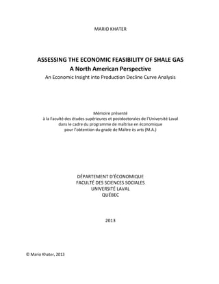
When production profiles in major gas regions are examined, what we generally see is a rising output
that peaks after a certain period of time, and then starts to decline to reach finally its economic limit (to
be defined later), even though there may still be a huge amount of the resource remaining in the ground
(Banks 2008). As showing in figure 6, after the decline phase, the play reaches its economic limit. At this
stage, no further production, nor economic or financial returns can still be expected. The reservoir (play)
is said to be out of pressure and no more gas can further be economically produced (Fekete associates
Inc. 2005).
Figure 6: Shale Gas Production Economics (Banks 2008)
Kaiser (2010) defines the economic limit of a reservoir as the time when the net revenue (gross revenue
net of royalty) of the field is equal to the field production cost (including taxes, operating and
transportation costs). To further extend the plateau, it may have a positive effect on the amount of gas
that can still be recovered, however, on the basis of reserves that have been recovered in a particular
deposit or field, it is uneconomical to attempt to prolonge the plateau indefinitely (Banks 2008).
Commonly, the biggest challenge in a shale gas investment is the capacity of operators to determine the
EUR of a shale reservoir. Since decline analysis is relatively simple, it was and will be adopted. Decline
curve analysis and EUR predictions are found in the public domain. Also, our analysis will be limited to
wells with publicly available data and will not include production improvements from workovers nor
recompletions or re-fracks.
Q (t)
Decline
Build-Up
Time
Costs
Economic limit
Clean-up Costs
Plateau
Additional investment

25
The first section of chapter II describes and explains the model, the methodology, and the model
economic parameters. The second section presents a comparative assessment of the economic
profitability of producing shale gas from five different shale plays (Barnett, Haynesville, Marcellus,
Montney, and Utica). Finally, the third section of our chapter introduces a logistic model that computes
various wells deployment scenarios within the industry in the Utica shale. Finally, conclusions and
recommendations will be advanced based on the results found.
2.1. Model, Methodology, Variables
Our study is conducted through decline curve analysis and breakeven economics. More precisely, the
profitability of shale gas production will be examined through cash flow sensitivity analysis. The main
purpose of evaluating the economics of shale gas projects is to calculate financial revenues that derive
from the production and the commercialization of shale gas under multiple development scenarios of
the industry. The same methodology is used by Lin (2010), Kaiser (2012), and Larry Lake, John Martin
and al. (2012).
2.1.1. Cash flow analysis
The importance of applying a cash flow analysis when assessing the economic feasibility of producing
shale gas is that it allows us to simulate and to test the impact of technical and financial inputs (to be
mentioned throughout the analysis) characteristics of shale gas economics on the anticipated financial
returns of the project.
Kaiser (2012) and Lake and al. (2012) point that the economic profitability of shale gas investments
should be tested by computing the total stream of after-tax net cash flows generated by the project. The
after-tax net cash flow is the difference between the estimated financial profits and the estimated
financial charges of the project over t periods, denoting the life span of the project. In our project, we
suppose that t = 20 years. Mathematically, the latter can be written as follows:
𝑁𝐶𝐹� = 𝑇𝑁𝑅� – (𝑅𝑂𝑌� + 𝐶𝐴𝑃_𝐸𝑋� + 𝑂𝑃_𝐸𝑋� + 𝐼𝑛𝑐_𝑇𝑎𝑥�) (1.4)
Where:
𝑁𝐶𝐹� denotes the after-tax net cash flow of the project (can be positive or negative), in year t, 𝑇𝑁𝑅�
denotes Total Nominal Revenues in year t, 𝑅𝑂𝑌� denotes Royalties paid in year t, 𝐶𝐴𝑃_𝐸𝑋� denotes
Capital Expenditures paid in year t, 𝑂𝑃_𝐸𝑋� denotes Operating Expenditures paid in year t, and finally,
𝐼𝑛𝑐_𝑇𝑎𝑥� denotes the corporate income tax rate paid in year t.
2.1.1.1. Explaining the model variables
When assessing the economic profitability of an investment project, a cash flow analysis consists on
computing the total stream of potential financial outcomes that could potentially be generated once the
project is brought on-line. The same logic applies to the assessment of the economics of shale gas
production.

26
Total Nominal Revenues in year t, 𝑇𝑁𝑅� denotes the potential financial profits that derive from the
launching of a shale gas project. The latter will be equal to the natural gas price 𝑝 paid in year t
multiplied by the volume of gas produced 𝑞� during the same year.
𝑇𝑁𝑅� = 𝑝 × 𝑞� (1.5)
To note that 𝑞� is estimated using Arps hyperbolic equation (1.2). Thus, if we replace 𝑞� by its value in
equation (1.5), we obtain:
𝑇𝑁𝑅� = 𝑝 × �𝑞� × (1 + 𝑏𝐷� 𝑡)�
�
�� (1.6)
Where 𝑝 and 𝑞� are two constants denoting natural gas price and initial production rate, respectively
and (1 + 𝑏𝐷� 𝑡)�
�
� is a function of time that we represent as 𝑓(𝑡). As a result, equation (1.6) can be
rewritten as:
𝑇𝑁𝑅� = (𝑝 × 𝑞�) × 𝑓(𝑡) = 𝛾 × 𝑓(𝑡) (1.7)
Equation (1.7) shows that if 𝑝 increases by two points (all other variables held constant), so will do
𝑇𝑁𝑅�. Any variation of 𝛾 implies that 𝑇𝑁𝑅� and 𝑞� will vary proportionally (linearly) over time. The value
of 𝛾 will depend upon two factors: (1) the economic environment under which firms choose to operate
and (2) the geologic properties of shale plays. To mention that we compute 𝑝 using the publically
available Henry Hub13
average prices forecasts. These forecasts show that average natural gas prices will
range between 2 and 8 dollars per mcf between 1990 and 2030.
As for Royalties 𝑅𝑂𝑌�. It represents a prospective cost to producing companies, generally a variable
fraction 𝜃 or financial charge to be paid to the government or to the land owner, per unit of production.
Mathematically, 𝑅𝑂𝑌� can be written as:
𝑅𝑂𝑌� = 𝜃 × 𝑞� (1.8)
Royalties can be found in the public domain and differ from a country (region) to another. Royalties in
the U.S. and Canada vary between 15 and 35% relatively to the amount of gas produced and sold
(Andrew Potter, Helen Chan and al. 2008). In Quebec (in the case of the Utica shale), the yearly fraction
of royalties that is to be paid to the government is largely dependent on annual volumes of gas
produced and prevailing natural gas prices. Quebec’s new royalty regime defines a range of 5-35% for
royalty rates.
The larger the volume of gas produced (the higher the price of gas) , the bigger the fraction of royalties
that will be paid and vice versa (Ministères des Finances 2011). Royalty rates specific to every shale play
will be defined later.
13
The Henry hub is a distribution hub on the natural gas pipeline system in Erath, Louisiana, owned by Sabine Pipe Line
LLC. The pricing is based on natural gas futures contracts traded on the New York Mercantile Exchange (NYMEX). Ref.:
Wikipedia.com.

27
Lake and al. (2012) points that in a shale gas project, drilling forms 60% of the total costs of producing
shale gas and completion forms the remainder 40%. Kaiser (2012) states that capital expenditures
consist of land acquisition, drilling and completion costs, pipeline infrastructure, etc. Kaiser (2012) also
mentions that those costs are the main costs in a shale gas production project. Hence, in our project,
capital expenditures, 𝐶𝐴𝑃_𝐸𝑋� will only consist of drilling and completion costs. In the analysis, we
suppose that 𝐶𝐴𝑃_𝐸𝑋� is a fixed cost or an initial investment cost that will be paid once at the launch of
the project ( 𝑡 = 0, 𝐶𝐴𝑃_𝐸𝑋� = 𝐶𝐴𝑃_𝐸𝑋). Capital expenditures specific to every shale play will be
specified later.
Operating expenditures or more precisely Lease Operating Expenditures (LOE) are defined as being the
costs that are associated with work physically performed at the work site (Kaiser 2012). In our project,
for simplicity purposes, we do not distinguish between the production of dry(cheaper)-wet(more
expensive) gas and we consider 𝑂𝑃_𝐸𝑋� as being a yearly (variable) cost, per unit of production. Finally,
the corporate income tax rate or simply the Income tax rate 𝐼𝑛𝑐_𝑇𝑎𝑥� is a yearly amount of money (a
fraction 𝜑 of 𝑁𝐶𝐹�) that is paid to the government once the production process of the resource has
started. Mathematically, 𝐼𝑛𝑐_𝑇𝑎𝑥� is computed as follows:
𝐼𝑛𝑐_𝑇𝑎𝑥� = 𝜑𝑁𝐶𝐹� (1.9)
In our project, we suppose an average taxation rate of 25% (Utica and Montney) (Lin 2010) and a range
of 30-50% (U.S. plays) (Kaiser 2012). In our analysis, we intentionally ignore some other types of costs,
such as: intangible costs, allowances, depletions costs, and we assume that those costs are directly
included in the initial investment cost ( 𝐶𝐴𝑃_𝐸𝑋) the reason why capital expenditures specific to every
shale play will be partially majorated in order to include those costs.
2.1.2. Sensitivity analysis
In most cases, in addition to the cash flow analysis, a sensitivity analysis of the project economics is
necessary to examine how the uncertainty in the model output can be allocated to various sources of
uncertainty in the model input (and vice versa). In our model, we define a base case development
scenario (average scenario, P50) for every shale play from which we launch our sensitivity analysis by
introducing an expected range for every shale gas input parameter. Thus, the average scenario (in terms
of production performance) will, at a certain extent, form the median of the expected range defined.
We also introduce two extreme case scenarios, an optimistic one (high development scenario, P10) and
a pessimistic one (low development scenario, P90), for every shale play, which are certainly less likely to
happen. In our study, we only use this nomenclature to categorize and represent well’s production
performances in terms of IP rate, Di rate and EUR.
More precisely, we define a set of P10, P50, and P90 scenarios for every shale play tested in our model
to represent wells with the best, average, and worst production performances, respectively.
This measure will allow us to define an upper and a lower bound for the calculated Net Present Value
(NPV) in every case (see, decision making indicators), allowing us eventually to compare the breakeven
economics of every shale play tested in our model.

28
To note that the sensitivity analysis will be applied to all three types of wells in every shale play. P10
profiles (wells) will obviously lead the most favorable economics and P90 the least favorable and the
results differential found will enable us to define profitability windows specific to every shale play. The
input ranges defined will vary from a shale play to another. Larger expected parameters ranges (inputs)
will be associated to larger amounts of uncertainty in the results (outputs) found.
Finally, the sensitivity analysis allows us to test the robustness of the results obtained in the cash flow
analysis. The sensitivity analysis input parameter combinations used are mainly three: (1) Gas Price and
IP rate (2) Gas Price and CAP_EX, and (3) Gas Price and CAP_EX to test the impact of -First Year Gas Price
(FYGP)- on P50 NPV project economics. The rest of the input parameters will be considered as static
over time. The outputs found in every case will be represented in Matrix-Tables and will be stated in
terms of NPV ($million), IRR (%), and Payout Period (years).
2.1.3. Decision making parameters
The economic indicators that will serve as decision making tools are three: (1) the NPV, (2) the IRR, and
(3) the payout period (or the economic limit of every shale play).
2.1.3.1. Net Present Value
The 𝑁𝑃𝑉 is the after-tax net stream of discounted cash flows ( 𝐷𝐶𝐹�) generated by the project. It uses
the time value of money to evaluate long term projects. It computes the excess or shortfall of cash
flows, in present value terms, once financial charges are met. Thus, it can serve as an investment
decision making tool. Generally, the investment options of a prudent company are three: Growth (Go),
Shutdown (No-Go) or temporary abandonment (conditional), respectively if the NPV is positive,
negative, or nil. Mathematically, the NPV can be represented as:
𝑁𝑃𝑉 = � 𝐷𝐶𝐹�
�
��
(1.10)
� 𝐷𝐶𝐹�
�
��
= �
𝑁𝐶𝐹�
(1 + 𝑟)�
�
��
(1.11)
And so, from equations (1.4), (1.10), and (1.11), we can write:
𝑁𝑃𝑉 = −𝐶𝐴𝑃_𝐸𝑋 + ��[𝑇𝑁𝑅� − (𝑅𝑂𝑌� + 𝑂𝑃_𝐸𝑋� + 𝐼𝑛𝑐_𝑇𝑎𝑥�)
�
��
] ×
1
(1 + 𝑟)�
� (1.12)
After rearranging equation (1.12) and replacing every variable by its expression, the mathematical
formula for the NPV can finally be represented as follows:
𝑁𝑃𝑉 = (1 − 𝜑) ��
[𝑝 − (𝑐 + 𝜃(𝑞�))] × 𝑞�
(1 + 𝑟)�
�
��
− 𝐶𝐴𝑃_𝐸𝑋� (1.13)

29
Where:
NPV denotes the after-tax net present value, (1 − 𝜑) denotes the 𝐼𝑛𝑐_𝑇𝑎𝑥� rate to be paid in year 𝑡 as a
fraction of the before-tax NPV generated in the same year; the latter is equal to the term showing in the
second parenthesis {…} on the right side of the equation,
�
(��)� denotes the discount factor ( 𝑟 denotes
the interest rate), [𝑝 − (𝑐 + 𝜃𝑞�)] × 𝑞� denotes the marginal profit of producing ( 𝑋 + 1) mcf of shale gas,
and (𝑐 + 𝜃𝑞�) computes all the variable costs (including operational costs, royalties, etc. as a function of
𝑞�) that the shale gas production process may imply.
Moreover, our analysis supposes one additional assumption stating that income taxes will only be paid if
𝑉 is positive. 𝑉 denotes the before-tax NPV. This assumption implies that the after-tax NPV will
potentially have two values depending on whether 𝑉 is positive or strictly negative:
𝑁𝑃𝑉 = �
(1 − 𝜑)𝑉 if 𝑉 ≥ 0
𝑎𝑛𝑑
𝑉 if 𝑉 < 0
� (1.14)
By developing and simplifying some of our model formulas, we made the correlational relationship
between our model input (Gas Price, IP rate and CAP_EX) and output parameters (NPV) clearer to see.
To note that the results of our NPV sensitivity analysis are all calculated based on both equations (1.13)
and (1.14).
2.1.3.2. Internal Rate of Return (IRR)
The 𝐼𝑅𝑅 is often used in capital budgeting and can be defined as the discount rate for which the
𝑁𝑃𝑉 = 0. Mathematically, the IRR is the annualised effective discount rate required for the NPV of a
stream of cash flows to equal zero therefore, equation (1.11) can be rewritten as follow:
𝑁𝑃𝑉 = �
𝑁𝐶𝐹�
(1 + 𝐼𝑅𝑅)�
�
��
= 0 (1.15)
Knowing that the 𝐼𝑅𝑅 is not affected by the 𝐶𝑜𝐶 (Cost of Capital) and the 𝐶𝑜𝐶 is a benchmark against
which the 𝐼𝑅𝑅 can be evaluated, comparing the 𝐼𝑅𝑅 to the 𝐶𝑜𝐶 should only be made when making
investment decisions. The calculated 𝐼𝑅𝑅 denotes the maximal acceptable value of 𝐶𝑜𝐶 for the project's
𝑁𝑃𝑉 to be profitable. If the 𝐼𝑅𝑅 > 𝐶𝑜𝐶 the project is said to be profitable (𝑁𝑃𝑉 > 0). However, if the
𝐼𝑅𝑅 < 𝐶𝑜𝐶 (𝑁𝑃𝑉 < 0), the project should not be undertaken. So, whilst a higher 𝐶𝑜𝐶 has zero impact on
the 𝐼𝑅𝑅, investment decisions will be rarely seen as profitable when using the 𝐼𝑅𝑅 as an indicator of
assessing those investment decisions.In our project, for simplify reasons, we suppose that a single firm
(Y) is exploiting all shale plays subject of our study and we assume that its 𝐶𝑜𝐶 is about 10% (relatively
to its debts and equities)14
.
14
Brealey R., Myers S. & Marcus A., Fundamentals of Corporate Finance, 3rd
Edition, McGraw-Hill, 2001.

30
In conclusion, investment decisions based on the calculated 𝐼𝑅𝑅 will depend upon the cost of capital
and the corporate objective of the firm as well as on its financial situation (financial exposure, solvability
& debt to equity ratios, etc.).
2.1.3.3. Payout Period
On an after-tax basis, payback period is simply the time 𝑇 required by the producing company to recover
all the prepaid financial charges that are associated with the project, mainly royalties and drilling and
completion costs (Kaiser 2010). However 𝑇 is uncertain and varies based on market and economic
conditions. Thus, it’s positively correlated with increases in gas prices and production levels, and vice
versa. So, while taking into account market and economic conditions, payback or payout periods denote
the earliest time required 𝑚 for the cumulative cash flow to recover well costs.
Mathematically, the payout formula can be written as follows:
𝑇 (years) = �� 𝐷𝐶𝐹� =
�
��
0� (1.16)
where 𝐷𝐶𝐹� denotes the vector of net cash flows in year 𝑡 [(𝑡 = 1, … , 20) 𝑦𝑒𝑎𝑟𝑠].
2.2. Shale plays and model assumptions
In this part of chapter II, a brief description of every shale play subject of our study will be proposed. We
also define shale plays model input parameters and their expected ranges. Our choice of the inputs and
their expected ranges will be justified throughout the analysis. The expected performances of every
shale play are summarized in Tables 1 (a, b, c, d, and e). The latter are collected from the public domain
and from various other academic sources.15
Tables 2 (a, b, c, d, and e) summarize the input parameters of shale plays and their expected ranges. To
add that our analyis is simply built on a after-tax basis and doesn’t assess the impact of income taxes on
the economic feasibility of shale plays and its only aim is to assess the economic feasibility of producing
shale gas from various shale plays under multiple development scenarios.
15
Engelder 2007; Andrew Potter, Helen Chan and al. 2008; Dan Magyar and Colin Jordan 2009; Jeff Ventura, Aubrey k.
McClendon and al. 2009; Bailey 2010; Lin 2010; Kaiser 2012; Larry Lake, John Martin and al. 2012; Mason 2012.

31
2.2.1. Barnett
The Barnett shale is a geological shale formation located in the Forth Worth Basin, Texas, U.S. The
formation is known as a tight gas reservoir indicating that the gas is buried almost 7000 feet deep and
cannot be easily extracted. Its estimated geographical extent is about 5000 square miles. The first
attempts of producing shale gas from the Barnett formation date from 1981. However, the effective
production of shale gas took place in 1999. This particular shale formation has been considered to have
significant underground gas reserves with almost 44 tcf of TRR and 327 tcf of GIP (González P. and al.
2012). Tables 1.a and 2.a present the expected performances for Barnett wells and its shale gas model
parameters and their expected ranges, respectively.
In Table 1.a, we define a set of initial production rates for Barnett wells based on three production
performance scenarios. We assume that P10 wells will have an IP rate of 5 Mmcf/day, P50 wells will
have a 3.5 Mmcf/day IP rate, and finally P90 wells will have an IP rate of 2 Mmcf/day. Our set of IP rates
is somehow justified by the fact that a typical Barnett well will have an IP rate of approximately 3.5
Mmcf/day (Jeff Ventura, Aubrey k. McClendon and al. 2009).
And so, P10 and P90 wells are basically set by defining a standard deviation of about ∓1.5 relatively to
P50 wells (median). The first year decline rate for Barnett wells is assumed to be the same for all well
performances and is set to 72%. The latter is merely higher than the decline rate used in Bailey (2010)
(66%) and merely lower than the one used by Ventura (2009) (73%). Decline rates for the rest of the
years are calculated using Arps equations. We also set a conservative range of EUR for every production
scenario.
Variable Code Unit P90 P50 P10
Initial production rate IP_rate Mmcf/d 2 3.5 5
Initial Decline rate ID_rate % per year 72 72 72
Estimated Ultimate Recovery EUR bcf per year 1.5 2 2.5
Table 2.a
Low Average High
Capital expenditures CAP_EX $million 4.5 3.5 2.5
Operational expenditures OP_EX $/mcf 1.5 1.25 1
Royalty rate Disc_rate % per year 25 25 25
Gas price GP $/mcf 2 5 8
Discount rate Disc_rate % per year 10 10 10
Corporate tax rate Inc_Tax % per year 30 30 30
Table 1.a Wells production performance
Barnett (Texas, U.S)
Development scenarios

32
Often, typical Barnett wells have an EUR of 2.5 bcf per year (Jeff Ventura, Aubrey k. McClendon and al.
2009). However, in our project we suppose that P10 wells will have an EUR of 2.5 bcf/year and P50 and
P90 wells will have 2 and 1.5 bcf/year of EUR, respectively. In Table 2.a we set a range for every input
parameter that characterizes the potential development scenario of the industry. We suppose that
𝐶𝐴𝑃_𝐸𝑋 will range between [2.5, 4.5] in million of dollars (2.5 is the minimum value that 𝐶𝐴𝑃_𝐸𝑋 can
take and 4.5 is its maximum possible value).
The average 𝐶𝐴𝑃_𝐸𝑋 scenario (3.5 million$) is set only to be used in the (𝐺𝑎𝑠 𝑃𝑟𝑖𝑐𝑒, 𝐼𝑃 𝑟𝑎𝑡𝑒) sensitivity
analysis. 𝐶𝐴𝑃_𝐸𝑋 is assumed to be the lowest under the high development scenario (P10) because it is
representative of the long run supply curve (growth) of the industry as a whole under which production
average costs will tend to decrease over time (know-how, advances in technology, economies of scale,
etc.) as long as the general level of gas produced and the marginal productivity of capital are increased.
This assumption is mainly representative of both external economies16
(positive externalities) and
economies of scale (cost advantages) long run concepts in the economic theory where factors of
production (capital, technology) will increasingly be incorporated into the production process leading to
higher production levels and eventually to lesser costs per unit produced. This particular assumption
applies to all shale plays subject of our study. To note that in our project 𝐶𝐴𝑃_𝐸𝑋 scenarios are
majorated to include some other costs such as: intangible costs, depreciation, etc. Ventura (2009) points
that capital expenditures for typical Barnett wells are about 2.3 million$ (horizontal wells only). We also
define a range of operating expenditures for the Barnett play of [1, 1.5] dollar per mcf of gas produced.
A similar range of 𝑂𝑃_𝐸𝑋� for the Barnett play can be found in (Bailey 2010), (Andrew Potter, Helen
Chan and al. 2008) and (Jeff Ventura, Aubrey k. McClendon and al. 2009). We also assume that the
royalty rate for the Barnett play is 25% on an annual basis17
. Finally, the tax on income was found in the
public domain and was somehow randomly set. For the Barnett play, we assume that the 𝐼𝑛𝑐_𝑇𝑎𝑥� is
about 30% per year.
16
Bourguinat Henri. Economies et déséconomies externes. In: Revue économique. Volume 15, n°4, 1964. pp. 503-532.
http://www.persee.fr/web/revues/home/prescript/article/reco_0035-2764_1964_num_15_4_407615.
17
http://blumtexas.tripod.com/barnettshalegas.html

35
2.2.2. Marcellus
The Marcellus formation is a sedimentary formation located in North Eastern America. It extensively
passes throughout the northern Appalachian basin and runs across the states of New York,
Pennsylvania, Virginia, Ohio, and Maryland. Its estimated geographical extent is 95000 square meters.
Typical Marcellus shale wells have initial production rates of about 4 Mmcf/day and EUR of 4.4 bcf. The
estimated TRR in this particular shale formation is 280 tcf and the GIP is estimated to be of about 1500
tcf (Engelder 2007; Jeff Ventura, Aubrey k. McClendon and al. 2009; González P. and al. 2012).
Before 2000, when the drilling started in the Marcellus formation, few experts thought that the
Marcellus shale would become a major source of natural gas. At first, wells drilled through it using
natural fractures systems produced gas in low quantities. Later on, with advances in technology,
Marcellus wells became economically productive and the Marcellus formation is now considered as the
giant gas field that will offset the future energy security concerns of the United States. Tables 1.b and
2.b below present the expected performances for Marcellus wells and shale gas model parameters and
their expected ranges, respectively.
In Table 1.b, we define a set of initial production rates for Marcellus wells based on three production
performance scenarios. We suppose an IP rate of 5 Mmcf/day for wells with highest production
performances, an IP rate of 4 Mmcf/day for wells with average production performances, and an IP rate
of 3 Mmcf/day for wells with lower production performances. The set of IP rates and EUR that are
associated to it can be found in Engelder (2007), Potter (2008) and Ventura (2009). We also assume that
the ID rate of typical Marcellus wells is 70% (Potter 2008). The latter applies to all development
scenarios.
Initial production rate IP_rate Mmcf/d 3 4 5
Table 2.b
Low Average High
Capital expenditures CAP_EX $million 5.5 4 2.5
Operational expenditures OP_EX $/mcf 1.1 1 0.9
Table 1.b
Marcellus (U.S)
Wells production performance

36
In Table 2.b, we set a range for every input parameter that characterizes the potential development
scenario of the industry. We suppose that 𝐶𝐴𝑃_𝐸𝑋 will range between [2.5, 5.5] million dollars. Potter
(2008) and Ventura (2009) assume that the average cost of drilling a single well in appalachia is almost 4
million$. Thus, in our project, we associate a 4 million$ 𝐶𝐴𝑃_𝐸𝑋 to the average development scenario
of the industry and we set a standard deviation of ∓1.5 relateviley to the average scenario in oder to
define 𝐶𝐴𝑃_𝐸𝑋 for high and low development scenarios, which are 2.5 and 5.5 million$, respectively.
Relatively to the case of the Barnett shale, we set lower operating costs for the Marcellus that range
between 0.9 and 1.1 $/mcf. Ventura (2009) sets operating costs in the Marcellus shale to 0.95$/mcf.
Generally, royalty rates are lower in appalachia relatively to other US shale plays. The majority of
Marcellus lands are freehold, with legislated royalties of 12.5 to 15% (Potter, 2008; Ventura, 2009). In
our project we adopt the upper bound royalty rate which is 15%. Finally, for simplicity reasons, we
assume that the tax rate on income is the same as it is the case for the Barnett shale (30% per year).

37
2.2.3. Haynesville
The Haynesville formation is a sedimentary formation that underlies thet states of Arkansas, Louisiana
and Texas from the south west to the northwest side of the United states. Its estimated geographical
extent is almost 9000 square miles. It contains 60 tcf of TRR. It came to scene and knew its boom in
2008. Since that date the Haynesville is seen as a major potential shale gas resource. Recently, some
experts have estimated that the Haynesville underground recoverable gas reserves are of the order of
250 tcf, and if true, the Haynesville would be considered as one of the largest natural gas fields in North
America (González P. and al. 2012).
Tables 1.c and 2.c showing below present the expected well performances for Haynesville wells and
shale gas model parameters and their expected ranges, respectively. Since 2008, the economics of the
Haynesville shale was extensively analyzed by several authors with or without economic and/or
academic affiliations, such as: Potter (2008), Kaiser (2010), Williams (2008), Kaiser (2012), and Lake and
al. (2012). In our project, the majority of Haynesville shale play model input parameters are found in
Kaiser (2012) and Lake and al. (2012).
We suppose that Haynesville P10, P50, and P90 wells have IP rates of 14 Mmcf/day, 11 Mmcf/day, and 8
Mmcf/day, respectively. Almost the same set of IP rates range can be found in Kaiser (2012), however,
our assumptions can be seen as relatively less optimistic. The same logic applies to the set of EUR that
we propose. Ventura (2009) supposes that the initial decline rate for Haynesville wells is 82%. As
showing in Table 1.c, we assume a merely higher ID rate of 85% for all types of wells.
In Table 2.c, we assume that capital expenditures for Haynesville wells range between 6 and 10 million
dollars. Kaiser (2012) points that capital expenditures for Haynesville wells range between 5 and 15
Estimated Ultimate Recovery EUR bcf per year 4.5 5.5 7
Table 2.c
Low Average High
Capital expenditures CAP_EX $million 10 8.5 6
Operational expenditures OP_EX $/mcf 2 1.5 1
Table 1.c Wells production performance
Haynesville (U.S)

38
million dollars. The latter is justified by the fact that we assume a lower IP rate (14 Mmcf/d) for
Haynesville P10 wells than it’s the case in Kaiser (2012) where P10 wells have a 16.1 Mmcf/d IP rate. For
operating expenditures, the same logic applies as it’s the case for 𝐶𝐴𝑃_𝐸𝑋, however, we only set a
narrower range for 𝑂𝑃_𝐸𝑋� and we assume that those costs will vary between 1 and 2 mcf/$.
We also assume a single, unchanging royalty rate of 25% for all Haynesville wells (Potter 2008; Ventura
2009; Kaiser 2012; Lake and al. 2012). Finally, we suppose a relatively high corporate tax rate of 45% per
year in the Louisiana region. The latter was set randomly from the range of corporate tax rates [35-50%]
found in Kaiser (2012) and could potentially affect or constraint the calculated Hayneville play NPV
project economics which should be understood.

39
2.2.4. Montney
The Montney formation is a 20,000 square feet natural gas field located in British Columbia, Canada, and
extends into Alberta (González P. and al. 2012). Natural gas can be found in large quantities trapped in
this shale play. Hence, the Montney shale play is seen to be according to a report by investment advisor
Raymond James Ltd, “one of the largest economically viable shale gas deposits in North-America”.
Moreover, according to the estimates of Halliburton, the Montney shale play probably contains 50 tcf of
GIP. Thus, since the early 2000’, a lot of producing companies like Talisman, Encana, Enersight and
others showed huge interest in having land leases to start exploring and drilling for shale gas in this
particular area.
Tables 1.d and 2.d below present the expected well performances for Montney wells and shale gas
model parameters and their expected ranges, respectively.
The ranges of IP rates and EUR that are associated with Montney P10, P50, and P90 wells was somehow
arbitraty set and so, the results found should be understood. A 6 Mmcf/day IP rate that is associated to
Montney P10 wells was taken from a best-fit production decline curve of Montney wells production
performances presented during the Unconventional Gas Confernce, CSUG, 2009. Thus, IP rates and EUR
showing in Table 1.d are not perfectly accurate and Montney wells could potentially register higher
initial production rates (and eventually have higher EUR) than those performances adopted in our
project. Moreover, all the other input parameters showing in both Tables 1.d and 2.d was taken from a
conference article of Enersight and BOE solutions presented during the same unconventional gas
conference in 2009 (Dan Magyar and Colin Jordan 2009).
Initial production rate IP_rate Mmcf/d 3 4.5 6
Estimated Ultimate Recovery EUR bcf per year 3 4.5 6
Table 2.d
Low Average High
Capital expenditures CAP_EX $million 9 7.5 5
Operational expenditures OP_EX $/mcf 2 1.5 1.5
Royalty rate Disc_rate % per year 23-35% 23-35% 23-35%
Table 1.d Wells production performance
Montney (BC, Canada)

40
According to Enersight, drilling a well in the Montney play costs 5.8 million dollars, and so based on this
fact, we have set a range of 𝐶𝐴𝑃_𝐸𝑋 scenarios between 5 and 9 million dollars for high and low
development scenarios, respectively. As already affirmed, 𝐶𝐴𝑃_𝐸𝑋 are majorated for the only purpose
of incorporating some other types of unaccounted costs. The same logic applies to 𝑂𝑃_𝐸𝑋�. According to
Enersight, those costs are strictly superior to 1$/mcf simplifying our choice of setting a range of
operating expenditures. In our project, we assume that 𝑂𝑃_𝐸𝑋� range between 1.5 and 2$/mcf.
For simplicity reasons, we assume that Montney’s natural gas is priced based on the Henry Hub, NYMEX
forecasts and not the AECO (Alberta Gas Trading Price). Magyar and Jordan (2009) points that the fiscal
model (in terms of royalty and tax regime) in Alberta range between 5 and 50% (an average royalty rate
of 22.5%). Thus, all along our analysis, we compute the economics of the Montney play while supposing
an average fixed royalty rate of 23% (≈22.5%) under all development scenarios. Finally, our choice of
corporate income tax (federal tax) was at certain degree arbitrary given that the fiscal system differs
between British Columbia and Alberta, so we had to choose among 2 different federal tax rates. We
offset this problem by setting a somehow average tax rate of 25%18
. Once again, the assumptions made
in the case of the Montney shale are somehow hazardous, especially those assumptions in terms of
federal taxes and royalty rates, and the results found should be understood.
18
Magyar, D. and Jordan, C., 2009. “Exploring the economics of a Montney Shale Gas Development on Both sides of the
border - BC versus Alberta”, Unconventional Gas Conference, CSUG, Well Spring.

41
2.2.5. Utica
The Utica shale basin is a sedimentary rock basin also known as “the Saint-Lawrence sedimentary basin”
located in Quebec, Canada. Since 2006, this particular shale formation started to gain real momentum
and to reveal some positive signs concerning its capacities to produce shale gas, economically. The latter
is estimated to have a geographical extent of about 2344 square miles and a GIP capacity of 25-160 bcf
per section (Lin 2010). Nowadays, the Utica shale is still in its early stages of development and its real
production capacities are still largely unknown. Tables 1.e and 2.e below present the expected well
performance for Utica wells and shale gas model parameters and their expected ranges, respectively.
We assume a 6 Mmcf/day and a 2 Mmcf/day IP rates for Utica P10 and P90 wells, respectively. The
latter data computes the exact IP rates registered by St-Edward and Gentilly wells drilled in the Utica
formation, respectively. EUR ranges and initial decline rates can be found in (Lin 2010). Lin (2010) point
that capital expenditures (drilling and completion costs) in the Utica play are most likely to vary between
5 and 7 million dollars and operating expenditures will often range between 1 and 2$ per mcf.
Thus, we assume that 𝐶𝐴𝑃_𝐸𝑋 vary between 5 and 7.5 million dollars which is logical and we adopt the
same range for 𝑂𝑃_𝐸𝑋� as it is assume in Lin (2010). In our project, we use in our calculation Quebec’s
new royalty regime. Previously royalty rates in Quebec varied between 10 and 12.5%. Presently,
according to the Ministères des Finances, royalty rates range between 5 and 35% depending on the
volume of gas produced and on prevailing natural gas prices19
. Finally, the corporate tax rate is set
19
Quebec’s new royalty regime will enter into force once the strategic environmental assessment (ÉES) that was
recommended by the BAPE has been completed and the legal and regulatory framework adapted to its conclusions.
Table 2.e
Low Average High
Capital expenditures CAP_EX $million 7.5 6 5
Operational expenditures OP_EX $/mcf 2 1.5 1
Royalty rate Roy_rate % per year 5-35% 5-35% 5-35%
Table 1.e Wells production performance
Utica (Québec, Canada)

42
randomly. We suppose that 25% is the yearly monetary fraction of gas produced and commercialized
that will go to the government.
Liu (2008) points that the combined federal and provincial income tax rate in Quebec amounts to 30.9%,
however, tax credits can eventually range between 20 and 40%. The latter shows that the fiscal regime
in Quebec is relatively more attractive when compared to other fiscal regimes in the U.S. and the rest of
Canada. The following part of our second chapter demonstrates and discusses the economic results of
our cash flow sensitivity analysis.
2.3. Economic discussion
Refer to Appendix (A.3. Results - Sensitivity Analysis). Technically, shale gas wells with high IP rates have
greater potentials to produce natural gas relatively to shale gas wells with lower initial production rates
(Jeff Ventura, Aubrey k. McClendon and al. 2009). Thus, based on our prefixed assumptions, Haynesville
wells will probably produce much more gas than it is the case for Marcellus wells, for example, and will
eventually register better economic performances. Nevertheless, higher initial decline rates mean that
the majority of cumulative gas production will come early in the life of the formation. Thus, the first 2
years of the life span of a gas well will be largely decisive of its economic feasibility. This is also mainly
the case of Haynesville wells.
The latter show the highest initial decline rates (85%) among other U.S. and Canadian shale plays.
However, this is not the case for Marcellus wells (and at a certain degree for Barnett wells), where,
whilst the production declines at a 70% rate after the first year, the latter will be associated to nothing
but to 7% of the total amount of gas that could be recovered.
Thus, longer reserve recoveries or lower recovery rates will largely impact the overall economics of the
play. In the case of Marcellus wells, much more time will be required to depict and evaluate the
production life cycle as well as the economic potential of the formation and this is mainly caused by the
existence of low recovery rates (Jeff Ventura, Aubrey k. McClendon and al. 2009). At this point, we
proceed by checking whether or not the results of our economic analysis will eventually come in
conformity with the above explanation of technical input parameters or else will show that the latter
characteristic of shale plays economics aren’t the only basis that delineate the economic profitability of
gas wells. The first (𝐺𝑎𝑠 𝑃𝑟𝑖𝑐𝑒, 𝐼𝑃 𝑟𝑎𝑡𝑒) sensitivity analysis table studies the impact of various market
and production scenarios on NPV economics of shale plays average development profiles.
Table 3 (silver line) shows that at an average development profile (in terms of costs), Marcellus and
Utica wells will have the lowest breakeven price (3$/mcf) followed by Barnett, Montney, and Haynesville
wells, respectively. The viability of these results will depend upon the assumptions made at the launch
of the analysis. However, a study conducted by Deutsche Bank in 2010, assessing the economics of five
different shale plays (Marcellus, Hayneville, Barnett, Fayetteville and Woodford), shows somehow a
similar result where Marcellus wells are estimated to have the lowest breakeven price (3.17$ per mcf)
when compared to other shale plays.

43
In a low economic environment where natural gas prices range between 2 and 4$/mcf, Montney and
Haynesville wells fail to breakeven on a half-cycle basis. The rest of the plays succeed to breakeven but
the registered NPV economics will relatively be low, and at a maximum wells performance scenario, only
Barnett and Marcellus wells succeed to register IRR that exceed the pre-fixed 10% cost of capital of the
producing company. More precisely, the IRR will be greater for the Marcellus than for other U.S. shales
and this will most probably derive from the existence of premium natural gas pricing due to location and
relatively low royalties in Appalachia. The same conclusion can be found in the Deutsche Bank report in
2010 and in Ventura (2009). The second (𝐺𝑎𝑠 𝑃𝑟𝑖𝑐𝑒, 𝐶𝐴𝑃_𝐸𝑋) sensitivity analysis assesses three wells
production performance profiles (P10, P50, and P90) NPV economics of shale plays under various
economic environments. Results found are summarized in Table 3 (blue line).
In a low economic environment, 2 $/mcf gas price, no value is created under most 𝐶𝐴𝑃_𝐸𝑋 scenarios for
all shale plays except for Marcellus P10 wells that could be brought in for less than 3 million dollars. For
P50 wells, profitability windows shrink and all shale plays fail to breakeven at a 2$/mcf gas price. At a
gas price of 4$/mcf, zero value is created for most shale plays except for Marcellus and Barnett P50
wells that can be brought in for less than 3.5 and 4.4 million dollars, respectively. However, at a gas
price of 6$/mcf, and under average 𝐶𝐴𝑃_𝐸𝑋 scenarios, almost all shale plays P50 wells succeed to
breakeven and to create value. Thus, a 6$/mcf represents a favorable economic environment and as
long as producing companies can maintain its drilling and completion costs at an average rate all shale
plays P50 wells will be marginally profitable.
Table 3: Shale plays breakeven prices ($ per mcf), under various input-parameters combinations:
*All the results (breakeven prices) computed in this table are rounded.
Shale_plays:
Marcellus Barnett Haynesville Montney Utica
4* 6* 5* 3*
3. P90 production profiles
(Gas Price , IP rate ):
-under average cost scenario-
5*
(Gas Price, CAP_EX ):
-Impact of First Year Price (FYP)-
2* 4* 6*
1. FYP (3$/mcf) and the rest
varies between 2 and 8$/mcf
2. FYP (8$/mcf) and the rest
varies between 2 and 8$/mcf
Sensitivity_Analysis_Results:
5*
4*
6*
2* 3*
7* 8*
3*
4*
3*
4*
2*
(Gas Price, CAP_EX ):
The combinations of
input_parameters tested:
3*

44
In a somehow moderate economic environment where gas prices range between 3 and 5 dollars per
mcf, most shale plays P10 wells succeed to breakeven if wells come at average 𝐶𝐴𝑃_𝐸𝑋 scenarios. More
precisely, at 5$/mcf, value is created for Marcellus, Barnett, and Utica P10 wells under all 𝐶𝐴𝑃_𝐸𝑋
scenarios and for almost all Haynesville and Montney P10 wells except those that can’t be brought in for
less than 10 and 8 million dollars, respectively. Finally, for all 𝐶𝐴𝑃_𝐸𝑋 scenarios depicted, all shale plays
P10 wells succeed to breakeven when gas prices range between 6 and 8$/mcf. At a 6$ per mcf gas price,
almost all Barnett and Marcellus P50 wells succeed to breakeven on a full 𝐶𝐴𝑃_𝐸𝑋 cycle. However, the
rest of shale plays P50 wells only succeed to breakeven under average 𝐶𝐴𝑃_𝐸𝑋 scenarios. Moreover, at
8$/mcf gas price and higher, all shale plays P50 wells succeed to breakeven and to create value. Table 3
(blue line) summarizes the breakeven prices of all shale plays P10, P50, and P90 wells, respectively.
Our analysis also shows that, under the most (𝐺𝑎𝑠 𝑝𝑟𝑖𝑐𝑒, 𝐶𝐴𝑃_𝐸𝑋) optimistic scenario, all shale plays
P10 wells succeed to breakeven in less than a one-year period. Furthermore, under the same optimistic
scenario, our sensitivity analysis results show that Marcellus P10 wells project economics register the
highest IRR (≈120%) followed by Barnett (≈93%), Hayneville (55%), Utica (54%), and Montney (50%) P10
wells. Finally, in a moderate economic environment where natural gas price is 5$/mcf, all shale plays
P90 wells fail to breakeven and to make money except for Marcellus wells that can be brought in for less
than 4.5 million dollars (exceeds the average development profile in terms of costs) which is most likely
unachievable.
In a more optimistic economic environment, where natural gas prices range between 6 and 8$/mcf, all
shale plays P90 wells succeed to breakeven (with relatively low NPV project economics) under low
𝐶𝐴𝑃_𝐸𝑋 scenarios except for Utica P90 wells that fail to breakeven under all 𝐶𝐴𝑃_𝐸𝑋 scenarios, none of
shale plays P90 wells succeed to breakeven and to create value under high 𝐶𝐴𝑃_𝐸𝑋 scenarios except for
Marcellus wells, and only few succeed to breakeven under average 𝐶𝐴𝑃_𝐸𝑋 scenarios (Haynesville,
Marcellus and Barnett).
Given the fact that shale gas production rates will decline steeply once the well is brought on-line; one
of the most important factors that will delineate the potential profitability of shale gas wells is the price
of the commodity during the first year of production (Kaiser 2012). In our last sensitivity analysis table,
we endeavor to assess the impact of first year prices (FYP) on all shale plays P50 wells NPV project
economics. We propose two (𝐺𝑎𝑠 𝑃𝑟𝑖𝑐𝑒, 𝐶𝐴𝑃_𝐸𝑋) scenarios where first year gas prices are 8$/mcf and
3$/mcf, respectively. The prices for the following years range between 2 and 8$/mcf. All other model
assumptions are the same as in (𝐺𝑎𝑠 𝑝𝑟𝑖𝑐𝑒, 𝐶𝐴𝑃_𝐸𝑋) sensitivity analysis for P50 wells.
Comparing results, we realize that profitability windows will increasingly expand for all shale plays when
gas prices are inferior to 8$/mcf. For example, Haynesville P50 wells register a NPV of 6 million$ at a
price of 8$/mcf when 𝐶𝐴𝑃_𝐸𝑋 are 6 million$. Taking the same (𝐺𝑎𝑠 𝑃𝑟𝑖𝑐𝑒, 𝐶𝐴𝑃_𝐸𝑋) combination, at a
first year gas price of 8$/mcf, Haynesville P50 wells almost register the same NPV level (5.9 million$).
However, if we consider the (5$, 6million$) combination, we realize that the NPV increases from 1.4$
million to 3.1$ million which is approximately an increase of 121% in NPV due to the first year price
differential.

45
Similarly, if we consider the case where the first year price is 3$/mcf (same 𝐶𝐴𝑃_𝐸𝑋 scenario), we realize
that the NPV decreases from -0.5 to -1.7 million$ which is approximately a decrease of 240% in NPV and
this decrease is also due to the first year price differential.
The same logic applies to all shale plays P50 NPV project economics whilst the impact can differ from
one play to another and the increase or decrease in NPV will depend upon several factors where the
most important one is the initial decline rate. Therefore, it’s most likely that the FYP will have the largest
impact on Haynesville P50 wells project economics (with the highest initial decline rate of almost 85%).
More precisely, the cumulative production curve of Haynesville wells shows that more than 25%
(
�
�.�
× 100) of GIP will be recovered during the first-year life span of the well and almost more than 73%
(
�.�
�.�
× 100) of GIP will be recovered in a 10-year period. Refer to appendix (A.4. Type Curves under 3
different production scenarios). Hence, it’s logical to say that higher or lower FYP will have the largest
impact on Haynesville wells NPV project economics (relatively to other shale plays). Table 3 (red line)
summarizes the impact of both 8$ and 3$/mcf first year prices on shale plays P50 wells breakeven prices
and shows the incremental value they provide.
On one hand, at a first year price of 8$ per mcf, all shale plays P50 wells succeed to breakeven under
high and average 𝐶𝐴𝑃_𝐸𝑋 scenarios. Profitability windows for all shale plays expand and almost all shale
plays P50 wells succeed to breakeven at a price of 2$ per mcf under low 𝐶𝐴𝑃_𝐸𝑋 scenarios at the
exception of both Montney and Utica P50 wells which breakeven at a price of 3$ per mcf.
Moreover, the analysis shows that at a FYP of 8$ per mcf Marcellus and Haynesville P50 wells show the
highest NPV increases followed by Utica, Barnett, and Montney P50 wells, respectively. On the other
hand, at a 3$/mcf FYP, the economic results are at a certain degree disastrous. Most of shale plays P50
wells fail to breakeven in a moderate economic environment under average 𝐶𝐴𝑃_𝐸𝑋 scenarios except
for Barnett and Marcellus P50 wells which breakeven at a price of 4$ and 2$/mcf, respectively. Under
high 𝐶𝐴𝑃_𝐸𝑋 scenarios, most of shale plays P50 wells fail to breakeven even under favorable economic
environments and only Barnett and Marcellus P50 wells succeed to breakeven at a price of 6$/mcf or
higher. Finally, at a 3$/mcf FYP, the profit window shrinks enormously for most P50 wells and even
those wells that succeed to breakeven will relatively generate insufficient economic returns to recover
the well and stimulate drilling and investment activities.

Economic Feasibility of Shale Gas

Economic Feasibility of Shale Gas

Recommandé

Recommandé

Contenu connexe

En vedette

En vedette (11)

Similaire à Economic Feasibility of Shale Gas

Similaire à Economic Feasibility of Shale Gas (20)

Economic Feasibility of Shale Gas