Scan Conversion Techniques for Lines and Polygons
•
0 j'aime•278 vues

Scan conversion algorithms convert graphical primitives defined in terms of coordinates into pixels on a raster display. The midpoint line algorithm uses integer calculations to scan convert lines of varying slopes. Area primitives like rectangles are filled by iterating through pixels within the boundary. Anti-aliasing aims to reduce jagged edges by weighting pixel intensities based on overlap with graphical elements.

Recommandé
Contenu connexe
Tendances
Tendances (20)
Similaire à Scan Conversion Techniques for Lines and Polygons
Similaire à Scan Conversion Techniques for Lines and Polygons (20)
Plus de Roziq Bahtiar
Plus de Roziq Bahtiar (20)
Dernier
Dernier (20)
Scan Conversion Techniques for Lines and Polygons
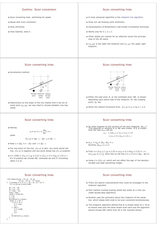
- 1. Outline: Scan conversion • Scan converting lines: optimising for speed. • Issues with scan conversion. • Area primitives. • How OpenGL does it. Scan converting lines • A more advanced algorithm is the midpoint line algorithm. • Does not use floating point arithmetic. • Generalisation of Bresenham’s well known incremental technique. • Works only for 0 ≤ m ≤ 1. • Other slopes are catered for by reflection about the principal axes of the 2D plane. • (x0, y0) is the lower left endpoint and (xe, ye) the upper right endpoint. Scan converting lines • Incremental method: M Q NE E Choices pixel current Choice for pixel Previous for next pixel • Restrictions on the slope of the line implies that if we are at some pixel (xp, yp), we now need to choose between only two pixels. Scan converting lines M Q NE E Choices pixel current Choice for pixel Previous for next pixel • Either the east pixel, E, or the northeast pixel, NE, is chosen depending upon which side of the midpoint, M, the crossing point, Q, lies. • Write the implicit functional from: f(x, y) = ax + by + γ = 0. Scan converting lines • Noting: y = mx + c = ∆y ∆x x + c , gives: f(x, y) = ∆y · x − ∆x · y + ∆x · c . • Now a = ∆y, b = −∆x and γ = ∆x · c. • For any point on the line, f(x, y) is zero, any point above the line, f(x, y) is negative and any point below has f(x, y) positive. • d = f(M) = f(xp + 1, yp + 1/2) = a(xp + 1) + b(yp + 1/2) + γ. If d is positive we choose NE, otherwise we pick E (including when d = 0). Scan converting lines • So what happens to the location of the next midpoint, Mnew? This depends on whether E or NE was chosen. If E is chosen then the new dnew will be: dnew = f(Mnew) = f(xp + 2, yp + 1/2) = a(xp + 2) + b(yp + 1/2) + γ . • dnew = dold + ∆E, ∆E = a. Similarly ∆NE = a + b. • First d = f(x0 + 1, y0 + 1/2) = a(x0 + 1) + b(y0 + 1/2) + γ = f(x0, y0) + a + b 2, since this on the line d = a + b/2 = ∆y − ∆x/2. • Using d = 2f(x, y), which will not affect the sign of the decision variable and keep everything integer. Scan converting lines void MidpointLine ( int x0, int xe, int y0, int ye, int value) { /* Assumes 0 <= m <= 1, x0 < xe, y0 < ye */ int x,y,dx,dy,d,incE,incNE; dx = xe - x0; dy = ye - y0; d = 2*dy - dx; incE = 2*dy; incNE = 2*(dy-dx); x = x0; y = y0; WritePixel(x,y,value); while (x < xe) { if (d <= 0) { d += incE; x++; } else { d += incNE; x++; y++; } WritePixel(x,y,value); } } Scan converting lines • There are several improvements that could be envisaged to the midpoint algorithm. • One method involves looking ahead two pixels at a time (so called double-step algorithm). • Another uses the symmetry about the midpoint of the whole line, which allows both ends to be scan converted simultaneously. • The midpoint algorithm defines that E is chosen when Q = M so to ensure lines look the same drawn from each end the algorithm should choose SW rather than W in the inverted version.
- 2. Line clipping NE y = y_min x = x_min M E • It is common to clip a line by a bounding rectangle (often the virtual or real screen boundaries). • Assume the bounding rectangle has coordinates, (xmin, ymin), (xmax, ymax). Line clipping NE y = y_min x = x_min M E • If the line intersects the left hand vertical edge, x = xmin the intersection point of the line with the boundary is (xmin, (m · xmin + c)). • Start the line from (xmin, Round(m · xmin + c)). Line clipping x = x_min y = y_min-0.5 y = y_min • Assume that any of the lines pixels falling on or inside the clip region are drawn. • The line does not start at the point ((ymin − c)/m, ymin) where the line crosses the bounding line. • The first pixel is Round (ymin − 0.5 − c) m , ymin . Line intensity • Lines of different slopes will have different intensities on the display, unless care is taken. • 2 lines, both 4 pixels but the diagonal one is √ 2 times as long as the horizontal line. • Intensity can be set as a function of the line slope. Scan converting area primitives void FillRectangle ( int xmin, int xmax, int ymin, int ymax, int value) { int x,y; for (y = ymin; y <= ymax; y++) { for (x = xmin; x <= xmax; x++) { WritePixel(x,y,value); } } } • Scan converting objects with area is more complex than scan converting linear objects, due to the boundaries. A rule that is commonly used to decide what to do with edge pixels is as follows. • A boundary pixel is not considered part of the primitive if the half-plane defined by the edge and containing the primitives lies below a non-vertical edge or to the left of a vertical edge. Filling polygons • Most algorithms work as follows: – find the intersections of the scan line with all polygon edges; – sort the intersections; – fill those points which are interior. • The first step involves the use of a scan-line algorithm that takes advantage of edge coherence to produce a data structure called an active-edge table. • Edge coherence simply means that if an edge is intersected in scan line i, it will probably be intersected in scan line i + 1. Other issues • Patterns will typically be defined by some form of pixmap pattern, as in texture mapping. • In this case the pattern is assumed to fill the entire screen, then anded with the filled region of the primitive, determining where the pattern can ‘show through’. • It is convenient to combine scan conversion with clipping in integer graphics packages, this being called scissoring. • Floating point graphics are most efficiently implemented by performing analytical clipping in the floating point coordinate system and then scan converting the clipped region. Scan conversion: OpenGL • OpenGL performs scan conversion efficiently behind the scenes – typically using hardware on the graphics card. • However, we can manipulate pixels using OpenGL with glRasterPos2i(GLint x, GLint y) and glDrawPixels(·) – in the labs you will code your own scan conversion routines. • Speed is often of the essence in computer graphics, so designing and developing efficient algorithms forms a large part of computer graphics research.
- 3. Anti-aliasing • All raster primitives outlined so far have a common problem, that of jaggies : jaggies are a particular instance of aliasing. The term alias originates from signal processing. • In the limit, as the pixel size shrinks to an infinitely small dot, these problems will be minimised, thus one solution is to increase the screen resolution. • Doubling screen resolution will quadruple the memory requirements and the scan conversion time. Anti-aliasing • One solution to the problem involves recognising that primitives, such as lines are really areas in the raster world. • In unweighted area sampling the intensity of the pixel is set according to how much of its area is overlapped by the primitive. • More complex methods involve weighted area sampling. • Weighted area sampling assumes a realistic model for pixel intensity. Using a sensible weighting function, such as a cone or Gaussian function, will result in a smoother anti-aliasing, but at the price of even greater computational burden. Anti-aliasing: OpenGL • Since anti-aliasing is an expensive operation, and may not always be required OpenGL allows the user to control the level of anti-aliasing. • Can be turned on using: glEnable(GL LINE SMOOTH) • Can also use glHint(GL LINE SMOOTH HINT,GL BEST) to set quality: GL BEST, GL FASTEST, and GL DONT CARE – hints not always implemented – based on number of samples. • Works by using the alpha parameter and colour blending. Anti-aliasing of polygons treated in the same way in RGBA mode. Summary • Having finished this lecture you should: – be able to contrast different approaches and sketch their application; – provide simple solutions to the problems of clipping and aliasing; – understand how scan conversion works in OpenGL.