1. ISA Transactions® Volume 45, Number 2, April 2006, pages 175–183
Adaptive predictive functional control of a class of nonlinear
systems
Bin Zhang* Weidong Zhang
Department of Automation, Shanghai Jiaotong University, Shanghai 200030, China
͑Received 8 March 2005; accepted 29 June 2005͒
Abstract
This paper describes the use of pseudo-partial derivative ͑PPD͒ to dynamically linearize a nonlinear system, and
aggregation is applied to the predicted PPD, resulting in a model-free adaptive predictive control algorithm for a
nonlinear system. The algorithm design is only based on the PPD derived online from the input/output data of the
controlled process, however it does provide bounded input/output sequence and setpoint tracking without steady-state
error. A detailed discussion on parameter selection is also provided. To show the capability of the algorithm, simulations
of a time-delay plant and a pH neutralization process show that the proposed method is effective for system parameter
perturbation and external disturbance rejection. © 2006 ISA—The Instrumentation, Systems, and Automation Society.
Keywords: Predictive functional control; Nonlinear system; Aggregation; Dynamic linearization; Base functions
1. Introduction The open literature presents a variety of nonlin-
ear control algorithms that are based on special
During the past decade the area of nonlinear nonlinear models such as Hammerstein model ͓1͔,
system control has been a forum for many re- Wiener model ͓2͔, and bilinear model ͓3͔, which
searchers. This is motivated to a large extent by have been at the forefront of nonlinear systems
the fact that nonlinear systems are difficult to con- research. However, it is difficult to find an appro-
trol, hence no general methods for algorithm de- priate nonlinear model “ f ” to describe the real pro-
sign are available. cess. Additionally, the nonlinear optimization
A discrete SISO nonlinear system can be typi- problem is rarely convex which adds to the diffi-
cally described by the following equation: culty of the online calculation. Therefore, re-
searchers turned to neural networks ͓4͔ which do
y P͑k + 1͒ = f ͑y P͑k͒, . . . ,y P͑k − ny͒,u͑k͒, . . . ,u͑k
satisfactorily map a bounded nonlinear function,
− nu͒͒ , ͑1͒ however there still exists the difficulty in real time
of a rapid, reliable application of the control algo-
where ny and nu are orders of outputs y P and in- rithm.
puts u, respectively, and f denotes a nonlinear More recently, the nonlinear function is assumed
mapping function. to be generalized Lipschitz with respect to output
and input, and a model-free learning adaptive al-
*Corresponding author. Tel: ϩ86.21.62826946; fax: gorithm is proposed by Hou and Huang ͓5͔ based
ϩ86.21.54260762. E-mail address: only on input and output information in which a
zhangbin7701@sjtu.edu.cn new concept called pseudo-partial derivative
0019-0578/2006/$ - see front matter © 2006 ISA—The Instrumentation, Systems, and Automation Society.

2. 176 B. Zhang, W. Zhang / ISA Transactions 45, (2006) 175–183
͑PPD͒ is used to linearize the nonlinear systems Assumption 2 (A2). The system is generalized
online. This idea was also used to develop an Lipschitz, that is, satisfying ͉⌬y P͑k + 1͉͒
adaptive-predictive PI controller ͓6͔. ഛ C͉⌬u͑k͉͒, for "k and ⌬u͑k͒ 0, where ⌬y P͑k
Model predictive control has been applied to + 1͒ = y P͑k + 1͒ − y P͑k͒, ⌬u͑k͒ = u͑k͒ − u͑k − 1͒ and
nonlinear processes ͓7–10͔, resulting in predictive C is a constant.
functional control ͑PFC͒ ͓11–14͔͒, which is a most The Lipschitz constant C is often required to be
promising model predictive control algorithm. The known for the control design purpose. Based on
PFC algorithm achieves computational simplicity the above assumption, the following result can be
by using simpler but more intuitive design guide- obtained.
lines ͓13͔ and in the past decade has been success- Theorem 1. ͓5͔ For the nonlinear system ͑1͒, we
fully used in industrial applications. The advan- assume that Assumptions ͑A1͒ and ͑A2͒ hold.
tages of fewer online calculations, a simpler Then there must exist G͑k͒, called PPD, when
algorithm and higher control precision are at- ⌬u͑k͒ 0,
tributes of the PFC, which contribute to its indus-
trial use. ⌬y P͑k + 1͒ = G͑k͒⌬u͑k͒ , ͑2͒
Motivated by the work of Hou and Huang ͓5͔
and Tan et al. ͓6͔, this paper presents an extension where
of PFC to nonlinear system control in which the
PPD concept is used to dynamically linearize the ͉G͑k͉͒ ഛ C ͑3͒
nonlinear system. In other words, the PPD re-
linearizes the nonlinear model as the plant moves With Theorem 1, Eq. ͑2͒ can be used as an internal
from one operating point to another, and uses the model to predict future process outputs
latest linear model as the internal model at each
step, resulting in solving a quadratic performance ˆ
͑QP͒. Aggregation as part of the algorithm ͓15͔ is
y ͑k + 1͒ = y ͑k͒ + G͑k͒⌬u͑k͒ , ͑4͒
used to predict future values of the PPD. Then
where
PFC is used to design the nonlinear adaptive con-
trol algorithm, in which only two coincidence
points are selected to calculate the manipulated ˆ
͉G͑k͉͒ ഛ C, ͑5͒
variable. The resultant controller has a simple
structure, hence tuning is not a problem. The pro- ˆ
y͑k͒ is the model output, and G͑k͒ is an estimate
posed algorithm can also provide bounded input/ of G͑k͒.
output sequences and track the setpoint without
steady-state error. Last, the paper discusses the pa-
rameter tuning, and uses simulations for a long 2.2. Predictive output and structured control
time delay plant and an experimental setup for the variables
measurement of the acidity or alkalinity in a Using Eq. ͑4͒, at sampling time k + Hi inside the
chemical reaction process to show that the pro- optimization horizon, the future output can be pre-
posed algorithm has higher precision and better dicted by
robustness to parameter perturbation than a PI or
PID controller. Hi
y ͑k + Hi͒ = y ͑k͒ + ͚ G͑k + j − 1͒⌬u͑k + j − 1͒ .
ˆ
j=1
2. Nonlinear adaptive predictive functional
͑6͒
control algorithm (NPFCA)
The PFC algorithm is different from other
2.1. The dynamic linearized internal model
model predictive controls. Instead of calculating
For a nonlinear system ͑1͒, the following two control signal with no restrictions, which may re-
assumptions are necessary: sult in an unstable control signal, PFC uses struc-
Assumption 1 (A1). The partial derivative of tured future manipulated variables, that is, the fu-
f͑·͒ with respect to the control input u͑k͒ is con- ture manipulated variables are parameterized by
tinuous. nB base functions uBj:

3. B. Zhang, W. Zhang / ISA Transactions 45, (2006) 175–183 177
nB inputs are calculated by minimizing the sum of the
u͑k + n͒ = ͚ ␮ j͑k͒uBj͑n͒ n = 0,1, . . . ,Hi − 1, quadratic difference between the predicted process
j=1 output and the reference trajectory at all coinci-
͑7͒ dence points. The criterion takes the following
form:
where ␮ j͑k͒ ͑j ෈ ͓1 , nB͔͒ are unknown coeffi-
H2
cients.
There are no restrictions for selecting these base min J P = ͚ ͓͑y ref͑k + n͒ − y ͑k + n͒ − e͑k + n͔͒͒2
n=H1
functions, and the selection of base functions has
no influence on the dynamic response or robust- M
ness and stability of the closed-loop system ͓12͔. + r ͚ ⌬u2͑k + n − 1͒ , ͑11͒
The base function can be selected as polynomial, n=1
sine, or exponential format. For many applications
where r is a weighting efficient, ͓H1 , H2͔ ͑H2
it is sufficient to describe the process input using a
Ͼ H1͒ is a coincidence horizon, M ͑M ഛ H2͒ is a
form such as u͑k + n͒ = ␮1͑k͒ + ␮2͑k͒n ͑n
control horizon, and e͑k + n͒ is the prediction error
= 0 , 1 , ¯ , Hi − 1͒, which results in
compensation which is given by e͑k + n͒ = e͑k͒
u ͑ k ͒ = ␮ 1͑ k ͒ , = y P͑k͒ − y͑k͒.
Substituting Eqs. ͑8͒–͑10͒ into Eq. ͑11͒, the cal-
⌬u͑k + Hi − 1͒ = ⌬u͑k + Hi − 2͒ = ¯ = ⌬u͑k + 1͒ culation of the process input u͑k͒ is straightfor-
ˆ
ward provided G͑k + j͒ is known. Note, Eq. ͑5͒
= ␮ 2͑ k ͒ . ͑8͒
ˆ
states that for "k , ͉G͑k͉͒ Ͻ C, require that future
Therefore, the determination of control input u͑k ˆ
predicted PPD G͑k + j͒ be bounded. To deal with
+ n͒ ͑n = 0 , 1 , ¯ , Hi − 1͒ means to find coeffi-
this restriction the idea of aggregation is adopted
cients ␮1͑k͒ and ␮2͑k͒ at each instant time k, and
ˆ
to predict future PPD at G͑k + j͒.
only u͑k͒ = ␮1͑k͒ is applied to the process.
Substituting Eq. ͑8͒ into Eq. ͑6͒ results in Let the aggregated variable be the current PPD
Gˆ ͑k͒, then future predicted values of the PPD
Hi
y ͑ k + H i͒ = y ͑ k ͒ + ͚ G ͑ k + j − 1 ͒ ␮ 2͑ k ͒
ˆ ˆ ˆ ˆ ˆ
͕G͑k + 1͒ , G͑k + 2͒ , . . . , G͑k + j͒ , . . . , G͑k + Hi − 1͖͒
j=2 can be described as the amplitude decaying se-
quence related to the aggregated variable, namely:
ˆ
+ G͑k͓͒␮1͑k͒ − u͑k − 1͔͒ ͑9͒
ˆ ˆ
G͑k + j ͒ = G͑k͒␭ j ͑0 Ͻ ␭ Ͻ 1, j = 1, ¯ Hi − 1͒
2.3. Optimization and control law equation ͑12͒
The PFC algorithm computes future process in- where ␭ is an unknown decaying coefficient.
put so that the predicted process output can follow ˆ
a reference trajectory. In the PFC algorithm, the Then, G͑k + j͒ can automatically meet the con-
reference trajectory is used to specify the desired straint requirement ͑5͒. Moreover, to facilitate the
future process behavior. For many applications a ˆ
tuning of the controller, this paper sets G͑k͒ = ␭,
first-order exponential reference trajectory is suf- then Eq. ͑12͒ can be modified to
ficient:
ˆ ˆ
G͑k + j͒ = ␭ j+1 = G͑k͒ j+1 ͑0 Ͻ ␭ Ͻ 1, j
y ref͑k + Hi͒ = w͑k + Hi͒ − ␩Hi͑w͑k͒ − y P͑k͒͒ ,
͑10͒ = 1, . . . ,Hi − 1͒ . ͑13͒
where ␩ = exp͑−Ts / Tref͒, Tref is the desired re- ˆ
However, the constraint for PPD G͑k͒ may cause
sponse time of the closed loop system, w is the an uncontrolled overshoot of ⌬u͑k͒, thus a weight
setpoint, and for constant value setpoint tracking for the control input ⌬u͑k͒ is introduced in the
w͑k + Hi͒ = w͑k͒. performance index Eq. ͑11͒. Since the control in-
The PFC algorithm requires an online optimiz- put ͑8͒ is used and the future predicted output is
ing method. When a QP index is used, the process given by Eq. ͑9͒, here we set M = H2.

4. 178 B. Zhang, W. Zhang / ISA Transactions 45, (2006) 175–183
For the assumption, ␮1͑k͒ and ␮2͑k͒ are un- e ͑ k + H 1͒ = e ͑ k + H 2͒ = y P͑ k ͒ − y ͑ k ͒ . ͑15͒
known coefficients in Eq. ͑11͒, which requires that
at least two coincidence points H1Ts and H2Ts
should be selected. Using Eq. ͑8͒, Eq. ͑11͒ is re- Substituting Eqs. ͑8͒–͑10͒, ͑13͒, and ͑15͒ into Eq.
written as ͑14͒, letting
min J P = ͓y ref͑k + H1͒ − y ͑k + H1͒ − e͑k + H1͔͒2
+ ͓y ref͑k + H2͒ − y ͑k + H2͒ − e͑k + H2͔͒2
‫ץ‬J P ‫ץ‬J P
M = 0, = 0. ͑16͒
‫ ͑1 ␮ ץ‬k ͒ ‫ ͑2 ␮ ץ‬k ͒
+ r͓␮1͑k͒ − u͑k͔͒ + r ͚
2
␮ 2͑ k ͒ ,
2 ͑14͒
n=2
where The manipulated variable is given by
ˆ ˆ ˆ ˆ
͓− A1G͑k͒ − A2G͑k͒ − ru͑k − 1͔͓͒S2 + S2 + r͑ M − 1͔͒ − ͑− A1S1 − A2S2͓͒S1G͑k͒ + S2G͑k͔͒
1 2
u ͑ k ͒ = ␮ 1͑ k ͒ = ,
ˆ ˆ ˆ
͓S G͑k͒ + S G͑k͔͒2 − ͓2G2͑k͒ + r͔͓S2 + S2 + r͑ M − 1͔͒
1 2 1 2
͑17͒
where Ai = w͑k + Hi͒ + ␩Hi͑w͑k͒ − y P͑k͒͒ + G͑k͒u͑k
− 1͒ − y P͑k͒ ͑i = 1 , 2͒,
ˆ
ˆ
͉G͑k͉͒ = ͯ ␥
␥ + ⌬u2͑k − 1͒
ˆ
G͑k − 1͒
Hi
+
⌬u͑k − 1͒
⌬y ͑k͒
␥ + ⌬u2͑k − 1͒ P
ͯ
Si = ͚ G͑k͒ j,
ͯ ͯ
ˆ ͑i = 1,2͒, M = H2 . ␥ ˆ
j=2 ഛ ͉G͑k − 1͉͒
␥ + ⌬u2͑k − 1͒
ͯ ͯ
ˆ
Subject to Eq. ͑4͒, online searching for G͑k͒ is
required, however in Eq. ͑2͒, many algorithms to ⌬u2͑k − 1͒
+ ͉G͑k − 1͉͒
ˆ
estimate G͑k͒ can be used. We adopted the adap- ␥ + ⌬u2͑k − 1͒
ˆ
tive learning algorithm ͓5͔ for G͑k͒: ␥ ⌬u2͑k − 1͒
ഛ C+ C = C.
␥ + ⌬u ͑k − 1͒
2
␥ + ⌬u2͑k − 1͒
͑19͒
ˆ ˆ ⌬u͑k − 1͒ ˆ
G͑k͒ = G͑k − 1͒ + ͑⌬y P͑k͒ − G͑k This inequality implies that the adaptive learn-
␥ + ⌬u2͑k − 1͒
ˆ
ing algorithm ͑18͒ for G͑k͒ also meets the con-
− 1͒⌬u͑k − 1͒͒ , ͑18͒
straint requirement ͑5͒.
Note that explicit control input constraints are
ˆ ˆ not addressed in this paper, however when input
where ␥ Ͼ 0, and the initial value G͑0͒ of G͑k͒
and/or state-related constraints need be consid-
are in the range of 0–1.
ered, the technique proposed by Abu el Ata-Doss
ˆ
Since ͉G͑k − 1͉͒ ഛ C and ͉G͑k − 1͉͒ ഛ C, it is ͓16͔ is usable.
easy to obtain the following relation with Eq. ͑18͒:

5. B. Zhang, W. Zhang / ISA Transactions 45, (2006) 175–183 179
3. Performance analysis of the closed loop Now we summarize the design procedure of the
control system and the algorithm proposed NPFAC as follows:
implementation Step 1: ͑Initialization͒ At time k = 0, take the ini-
ˆ ˆ
tial value G͑0͒ of PPD G͑k͒ are in the range of
In order to assure the convergence of the closed 0–1, and set ␥ Ͼ 0.
loop system, the following assumption is made. Step 2: Find appropriate coincidence points
Assumption 3 (A3): The PPD satisfies G͑k͒ H1 , H2, and the closed-loop response time Tref by
Ͼ 0 for "k. using the criterion ͑A4͒ and ͑21͒. Further, for a
Based on the previous assumption, the stability time delay system both the two coincidence points
of the closed loop system is guaranteed in the fol- H1 and H2 should be selected larger than the dead-
lowing theorem. time in samples. Set the input horizon M = H2 and
Theorem 2: Subject to Assumptions ͑A1͒–͑A3͒, the weighting coefficient r to verify inequality
the algorithm Eq. ͑17͒ for the nonlinear system ͑A6a͒.
Eq. ͑1͒ is used to track the setpoint w, then coin- Step 3: At time k ജ 1, collect the process input/
cidence points Hi͑i = 1 , 2͒, the weighting coeffi- ˆ
output data, and find G͑k͒ by using adaptive learn-
cient r Ͼ 0, and the control horizon M = H2 Ͼ 1 ex- ˆ
ist such that ing algorithm ͑18͒. Substitute G͑k͒ into ͑A4͒,
͑A6a͒, and ͑21͒, if these three conditions fail, re-
lim ͉y P͑k + 1͒ − w͉ = 0 ͑20͒ turn to Step 2. Otherwise, go to Step 4.
k→ϱ
Step 4: Use the control law equation ͑17͒ to cal-
and ͕y P͑k͖͒ , ͕u͑k͖͒ are bounded sequences. culate the process control input and apply it to the
Proof: See the Appendix. process.
Note, the G͑k͒ in Eq. ͑A6b͒ is unknown at cur- Step 5: At the next point, repeat Steps 3 and 4.
rent time k and G͑k͒ Ͻ C. If we take the following
inequality as a criterion for selecting controller pa- 4. Illustrative examples
rameters, then the condition ͑A6b͒ always holds
The following long time delay plant and pH
G͑k͒2 Ͼ CG͑k͒͑1 − ␩Hi͒ ͑i = 1,2͒ .
ˆ ˆ ͑21͒ measurement of acidity or alkalinity process are
Theorem 2 actually provides a criterion to select used to show the effectiveness of the proposed al-
controller parameters. That is, existing parameters gorithm.
r Ͼ 0, Hi͑i = 1 , 2͒, and M = H2 Ͼ 1 insure that Eqs. Example 1: Consider a plant described by
͑A4͒, ͑A6a͒, and ͑21͒ are applicable. Further, from K
Eq. ͑A3͒ increasing r leads to ␳ decreasing, and P͑s͒ = e −␪s ͑22͒
͑s + 1͒3
Eq. ͑A2͒ shows that increasing r results in a
slower tracking of the setpoint. Theorem 2 also in which K = 1 and ␪ = 15. Our goal is to use the
shows that Tref has no influence on stability. The proposed NPFCA to control such a large time-
rapidity of Tref will influence the dynamic re- delay plant and to show that the proposed control
sponse and robustness of the closed-loop system. method gives a better performance than a PI or
The shorter Tref, the more active the controller will PID controller. A comparison to the methods of
be with larger amplitude variations ͓12͔. Astrom-Hagglund’s PI tuning ͑A-H PI͒ ͓17͔, Sig-
ˆ urd Skogestad’s IMC-PI and IMC-PID tuning
Note that parameter estimation for G͑k͒ is con-
͑SIMC-PI, SIMC-PID͒ ͓18͔ is given. Using the
vergent and the coincidence points H1 , H2, the in-
above-mentioned tuning methods, the recom-
put horizon M = H2, the weighting coefficient r,
mended controller parameters are as follows:
and the reference trajectory time Tref are easily
selected using Eqs. ͑A4͒, ͑A6a͒, and ͑21͒. Since A-H PI: Gc͑s͒ = 0.2115 + 0.0286/s
the developed method has no plant structural re-
quirement, the closed-loop control scheme is very SIMC-PI: Gc͑s͒ = 0.0455͑1 + 1/1.5s͒
ˆ
robust. In practice, H1 , H2, the initial value G͑0͒,
SIMC-PID: Gc͑s͒ = 0.0322͑1 + 1/s͒͑1 + 1.5s͒
and Tref can be fixed, and r is used to tune so that
an optimal compromise between performance and For the proposed NPFCA, we choose the sam-
robustness can be reached. pling time Ts = 1 s. Follow the design procedure in

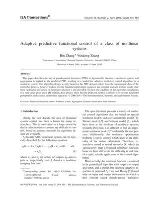
6. 180 B. Zhang, W. Zhang / ISA Transactions 45, (2006) 175–183
Fig. 1. Step responses of the nominal closed loop system. Fig. 2. Step responses of the perturbed closed loop system.
ˆ
Section 3, we take the initial value of PPD G͑0͒ and disturbance rejection. Further, it is easy to
= 0.9, and ␥ = 0.9. In Step 2, since the plant con- verify that at each sampling time for the proposed
sidered contains a large time delay, the coinci- controller parameters the conditions ͑A4͒, ͑A6a͒,
dence points H1 and H2 should be selected larger and ͑21͒ always hold.
than the dead-time. Then by Eqs. ͑A4͒, ͑A6a͒, and Fig. 2 shows the responses to process parameter
͑21͒, the controller tuning parameters used here perturbation: K = 1.3 and ␪ = 16. Note that the
are assigned at coincidence points H1 = 20, H2 SIMC-PI and SIMC-PID methods are very oscil-
= 22, the input horizon M = H2 = 22, the desired latory, and A-H method provides poor disturbance
closed-loop response time Tref = 1 s, and the rejection. The proposed method provides a smooth
weighting coefficient r = 75. setpoint response and an acceptable disturbance
For a step change in the unit setpoint and a load rejection. The improvement on performance is due
disturbance at t = 0 s and t = 185 s, respectively, to that the proposed algorithm has no plant struc-
Fig. 1 presents these step responses of the closed- tural requirement and adopts an adaptive learning
loop control system. One can see that for setpoint algorithm to on-line estimate PPD G͑k͒.
changes, as well as disturbance inputs the A-H PI Example 2: A pH neutralization process can be
method, SIMC-PI, and SIMC-PID methods do not modeled by the following equation ͓14͔:
reach the final set point at about time t = 300 s, x͑k͒ = f 1͑u͑k͒͒ = u͑k͒ − ͑1.207 + r1͒u2͑k͒
whereas the newly developed method provides
significant improvement in both setpoint response + 1.15u3͑k͒ , ͑23a͒
y ͑k͒ ͑0.0185 + r2͒z−2 + ͑0.0173 + r3͒z−3 + 0.00248z−4
= , ͑23b͒
x͑k͒ 1 − ͑1.558 + r4͒z−1 + 0.597z−2
where r1, r2, r3, and r4 are time-varying param- It can be found that the proposed method does
eters of the process in which the initial values are achieve excellent results. Fig. 4 shows the re-
set to zero. Selecting the initial value of the PPD sponse to a unit output disturbance at time t
ˆ
to G͑0͒ = 0.98, ␥ = 0.9, coincidence points H 1
= 250 s with no change in controller parameters.
= 17, H2 = 25, the input horizon M = 25, the sam- Again the proposed controller performs very well.
pling time Ts = 1 s, the desired closed loop re- The proposed control system can track setpoint
sponse time Tref = 1 s, and r = 300, the step re- without steady-state error although there is an ex-
sponses for setpoint tracking are shown in Fig. 3. isting external disturbance. In addition, for the

7. B. Zhang, W. Zhang / ISA Transactions 45, (2006) 175–183 181
Fig. 3. Output ͑top͒ and input ͑bottom͒ of the closed loop Fig. 5. Step response of the closed loop system with time-
step responses for setpoint tracking. varying parameters.
case of process parameter perturbation occurring structure of the plant or any further external forc-
at different times t = 200 s ͑r1 = 0.1, r2 = 0.01͒ and ing for purposes of model development. Note, the
t = 400 s ͑r3 = 0.001, r4 = −0.008͒, the step re- results presented in this paper can be extended to
sponse is shown in Fig. 5. One can see that the MIMO nonliner processes, and the proposed
proposed algorithm has excellent robustness. scheme can be easily implemented.
5. Conclusions
Appendix: Proof of theorem 2
The PPD was used to dynamically linearize a
nonlinear process, and aggregation was used to For constant value setpoint tracking, the error
predict the PPD, resulting in an adaptive predic- between the output y P and the constant setpoint w
tive functional control algorithm ͑APFCA͒ for can be written as follows:
nonlinear processes. The proposed algorithm was E ͑ k + 1 ͒ = ͉ y P͑ k + 1 ͒ − w ͉ = ͉ y P͑ k ͒ − w
tested on two processes and was shown to clearly
outperform existing algorithms. + G͑k͒⌬u͑k͉͒ = ͉y P͑k͒ − w + G͑k͒͑u͑k͒
A theorem, which illustrates that the designed
control system can track the setpoint with zero er- − u͑k − 1͉͒͒ . ͑A1͒
ror and input/output sequences are bounded, was Substituting Eq. ͑17͒ into Eq. ͑A1͒ results in Eq.
derived in this paper. A merit of the proposed con- ͑A2͒.
troller algorithm is that it does not require the
E͑k + 1͒ ഛ ͉1 − ␳͉E͑k͒ , ͑A2͒
where
␰
␳=
␷
␰ = G͑k͒G͑k͒͑S2 − S1͓͒͑1 − ␩H1͒S2 − ͑1 − ␩H2͒S1͔
ˆ
+ G͑k͒G͑k͒r͑ M − 1͒͑2 − ␩H1 − ␩H2͒ ,
ˆ
ˆ ˆ
␷ = G2͑k͒͑S2 + S2 − 2S1S2͒ + ͓2G2͑k͒ + r͔r͑ M − 1͒
1 2
+ rS2 + rS2 .
1 2 ͑A3͒
Fig. 4. Step response of the closed-loop system with output
From Assumption 3 and Eq. ͑18͒, it is easy to
disturbance. ˆ
know that G͑k͒ Ͼ 0. Note, S2 Ͼ S1, Assumption 3

8. 182 B. Zhang, W. Zhang / ISA Transactions 45, (2006) 175–183
ˆ
states G͑k͒G͑k͒ Ͼ 0, and Eq. ͑10͒ shows that 0 G͑k͒2 Ͼ G͑k͒G͑k͒͑1 − ␩Hi͒͑i = 1,2͒ .
ˆ ˆ
ഛ ͑1 − ␩ ͒ Ͻ 1͑i = 1 , 2͒, therefore, if we set r Ͼ 0,
Hi
M = H2 ജ 1, and Hi͑i = 1 , 2͒ such that ͑A6b͒
Then ␷ Ͼ ␰ Ͼ 0, and is ␳ = ␰ / ␷ Ͻ 1, and 0 Ͻ 1 − ␳
͑ 1 − ␩ H1͒ S 2 Ͼ ͑ 1 − ␩ H2͒ S 1 ͑A4͒ Ͻ 1.
By Eq. ͑A2͒, the following inequality holds:
results in ␳ Ͼ 0.
E ͑ k + 1 ͒ ഛ ͉ 1 − ␳ ͉ E ͑ k ͒ ഛ ͉ 1 − ␳ ͉ 2E ͑ k − 1 ͒ ഛ ¯
Furthermore, from Eq. ͑A3͒ one can derive Eq.
͑A5͒. ഛ ͉1 − ␳͉k+1E͑0͒ . ͑A7͒
Then
␷ − ␰ = S2͓G͑k͒2 − G͑k͒G͑k͒͑1 − ␩H2͔͒ + S2͓G͑k͒2
1
ˆ ˆ
2
ˆ
lim ͉y P͑k + 1͒ − w͉ = lim E͑k + 1͒
2 k→ϱ k→ϱ
− G͑k͒G͑k͒͑1 − ␩H1͔͒ + ͚ ͓G͑k͒2
ˆ ˆ
i=1 = lim ͑1 − ␳͒k+1E͑0͒
k→ϱ
− G͑k͒G͑k͒͑1 − ␩Hi͔͓͒r͑ M − 1͒ − S1S2͔
ˆ ͑A8͒
+ r 2͑ M − 1 ͒ + r ͑ S 2 + S 2͒ .
1 2 ͑A5͒ Since 0 Ͻ 1 − ␳ Ͻ 1 and E͑0͒ = ͉y P͑0͒ − w͉ = ͉w͉, it
is easy to know by ͑A8͒ that Eq. ͑20͒ holds and
If r Ͼ 0, M = H2 Ͼ 1, and Hi͑i = 1 , 2͒ are selected the control system track setpoint with no steady
such that state error.
Moreover, we use the following form for ␳1:
r ͑ M − 1 ͒ Ͼ S 1S 2 ͑A6a͒ ␳ = G͑k͒␳1 , ͑A9͒
and where
G͑k͒͑S2 − S1͓͒͑1 − ␩H1͒S2 − ͑1 − ␩H2͒S1͔ + G͑k͒r͑ M − 1͒͑2 − ␩H1 − ␩H2͒
ˆ ˆ
␳1 =
ˆ ˆ
G2͑k͒͑S2 + S2 − 2S S ͒ + ͓2G2͑k͒ + r͔r͑ M − 1͒ + rS2 + rS2
1 2 1 2 1 2
and a bound for ␳ and G͑k͒ exist, ␳1 will be ͉u͑k͉͒ ഛ ͉u͑k͒ − u͑k − 1͉͒ + ͉u͑k − 1͉͒
bounded.
Combing Eqs. ͑17͒ and ͑A3͒ resulting in ഛ ͉⌬u͑k͉͒ + ͉u͑k − 1͒ − u͑k − 2͉͒ + ͉u͑k − 2͉͒
ഛ ¯ ഛ ͉⌬u͑k͉͒ + ͉⌬u͑k − 1͉͒ + ¯
⌬u͑k͒ = u͑k͒ − u͑k − 1͒ = ␳1͓w − y P͑k͔͒ + ͉⌬u͑2͉͒ + ͉u͑1͉͒ ͑A12͒
͑A10͒ Thus by Eq. ͑A11͒ ͕y P͑k͖͒, ͕u͑k͖͒ are bounded
sequences.
and ᮀ
͉⌬u͑k͉͒ ഛ ␳1maxE͑k͒ ͑A11͒ Acknowledgments
where ␳1max is the upper bound of ␳1. Using the The authors would like to thank the National
absolute triangle inequality property to Eq. ͑A10͒, Natural Science Foundation of China ͑60274032͒,
it results, Specialized Research Fund for the Doctoral Pro-

9. B. Zhang, W. Zhang / ISA Transactions 45, (2006) 175–183 183
gram of Higher Education ͑SRFDP͒ partial least squares. Chem. Eng. Res. Des. 80, 75–86
͑20030248040͒ for financial support of the re- ͑2002͒.
͓9͔ Kwon, Wook Hyun, Han, SooHee, and Ahn, Choon
search project. Ki, Advances in nonlinear predictive control: A survey
on stability and optimality. International Journal of
References Control, Automation and Systems 2, 15–22 ͑2004͒.
͓10͔ Qin, S. J. and Badgwell, T. A., An overview of non-
͓1͔ Fruzzetti, K. P., Palazoglu, A., and McDonald, K. A., linear model predictive control applications. Nonlinear
Nonlinear model predictive control using Hammer- Model Predictive Control, edited by Allgöwer, F. and
stein models. J. Process Control 7, 31–41 ͑1997͒. Zheng, A., Birkhäuser, Switzerland, 2000.
͓2͔ Norquay, S. J., Palazoglu, A., and Romagnoli, J. A., ͓11͔ Richalet, J., Industrial application of model based pre-
Application of wiener model predictive control dictive control. Automatica 29, 1259–1274 ͑1993͒.
͑WMPC͒ to a pH neutralization experiment. IEEE ͓12͔ Ernst, T. E. F. H. C., First principle modeling and pre-
Trans. Control Syst. Technol. 7, 437–445 ͑1999͒. dictive functional control of enthalpic processes, Ph.D.
͓3͔ Daniel-Berhe, S. and Unbehauzn, H., Bilinear thesis, Delft University of Technology, Delft, The
continuous-time systems identification via hartley- Netherlands, 1996.
based modulating functions. Automatica 4, 499–503 ͓13͔ Rossiter, J. A. and Richalet, J., Handing constraints
͑1998͒. with predictive functional control of unstable pro-
͓4͔ Zhang, J., Developing robust non-linear models cesses. Proceedings of the American Control Confer-
through bootstrap aggregated neural networks. Neuro- ence, Anchorage, Alaska, 4746–4751, 2002.
computing 25, 93–113 ͑1999͒. ͓14͔ Zhang, Q. L., Predictive functional control and its ap-
͓5͔ Hou, Z. S. and Huang, W. H., The model-free learning plications. Ph.D thesis, Zhejiang University, 1999.
adaptive control of a class of SISO nonlinear systems. ͓15͔ Xi, Y. G., The principles and methods in large scale
Proceedings of the American Control Conference, dynamical systems. National Industry Press, 1988.
New Mexico, 343–344, 1997. ͓16͔ Abu el Ata-Doss, S., Finai, P., and Richalet, J., Hand-
͓6͔ Tan, K. K., Huang, S. N., Lee, T. H., and Leu, F. M., ing input and state constraints in predictive functional
Adaptive-predictive PI control of a class of SISO sys- control. Proceedings of the 30th Conference on Deci-
tems. Proceedings of the American Control Confer- sion and Control, Brighton, 985–990, 1991.
ence, California, 3848–3852, 1999. ͓17͔ Astrom, K. J. and Hagglund, T., Industrial adaptive
͓7͔ Maqni, L. and Scattolini, R., Stabilizing model predic- controller based on frequency response techniques.
tive control of nonlinear continuous time systems. Automatica 27, 599–600 ͑1991͒.
Annu. Rev. Control 28, 1–11 ͑2004͒. ͓18͔ Skogestad, S., Simple analytical rules for model re-
͓8͔ Baffi, G., Morris, J., and Martin, E., Non-linear model duction and PID controller tuning. J. Process Control
based predictive control through dynamic non-linear 13, 291–309 ͑2003͒.