Correlation (mutual relation of two or more things) and Linear Regression

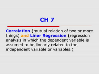
1. CH 7
Correlation (mutual relation of two or more
things) and Liner Regression (regression
analysis in which the dependent variable is
assumed to be linearly related to the
independent variable or variables.)

2. Learning Objectives
1) How to use correlation analysis to
describe the relationship between twotwo
interval-levelinterval-level variablesvariables.
2) How to use regression analysis to
estimate the effect of an independent
variable on a dependent variable.
3) How to perform and interpret dummy
variable regression.
4) How to use multiple regression to make
controlled comparisons.

3. Book has covered fair amount of methodological ground.
 Ch 3 learned two essential methods for analyzing
relationship between an independent variable and a
dependant varb: 1) cross-tabulation 2) mean comparison
analysis.
 Ch 4 covered the logic and practice of controlled comparison
– how to set up and interpret the relationship between an
indp variable and a dep varb, controlling for a third variable.
 CH’s 5 and 6 learned of role of inferential statistics in
evaluating the statistical significance of a relationship, and
became familiar with measures of association.
 By now, you can: 1) frame a testable hypothesis; 2) set up
the appropriate analysis; 3) interpret your findings; 4) and
figure out the probability that you observed results occurred
by chance.

4. In many ways, correlation and regression are similar to the
methods you have learned.
 Correlation analysis = produces a measure of association –
Pearson’s correlation coefficient which gauges the direction
and strength of a relationship between two interval-level
variables.
 Regression analysis = produces a statistic, a Regression
Coefficient, that estimates the size of the effect of the
independent variable on the dependant variable.
 Emp = Working with survey data, want to investigate the relationship
between individuals’ ages (Indep Varb) and number of hours they
spend watching television each day (Dep Varb).
 1) Is the relationship positive, with older indivduals watching more hours of TV.
 2) Is the relationship negative, with older people watching less TV than younger
people.
 3) How strong is the relationship between age and number of hours devoted to
TV?
 Correlation analysis addresses theses questions.

5. Regression analysis is similar to mean comparison analysis:
1) where we learned to divide subjects on the independent variable:
females and males.
2) And how to compare values on the dependent variable, – like the
mean Clinton thermometer ratings.
3) Furthermore, learned how to test the null hypothesis with
assumption of random sampling error.
 Similarly, Regression Analysis communicates mean difference on
the dependent variable (thermometer ratings) for subjects who differ
on the independent variable, females compared with males.
 Just like comparison of two sample means, Regression Analysis
provides info that permits the researcher to determine the
probability that the observed difference was observed by chance.

6. However, regression is different in two ways:
 1) Regression analysis is very precise. It provides the statistic, the
Regression Coefficient that reveals the exact nature of the relationship
between an indp varb and a dep varb.
 Regression coefficient reports “the amount of change in the dep varb that is
associated with a one-unit change in the indp varb.”
 Regression coefficient is used only when the dep varb is measured at the
interval level.
 The independent varb can come in any form: nominal, ordinal, or interval.
 In ch, we show how to interpret regression analysis in which the indep varb is interval
level.
 Also, CH discusses technique called dummy variable regression – uses nominal or ordinal
varbs as indp varbs.
 2) A second distinguishing feature of Regression is the ease it can be
extended to the analysis of controlled comparisons.
 Regression also analyzes the relationship between a dependent varb and a
single indep varb – Bivariate Regression = One Indep Varb and one Dep Varb.
 Regression is remarkably flexible, it can be used to detect and evaluate
spuriousness, and it allows us to model additive relationships and interaction

7. Correlation
 Eamp in Book: The relationship between two variables: % of a state’s
population that graduated from high school ( indep varb), and % of
eligible pop that voted in the 1994 elections (dep varb). Display is a
Scatterplot = the indp varb is measured along the horizontal axis and
the dep varb is measured along the vertical axis.
 Consider the overall pattern of this relationship: 1) Is it strong, moderate, or weak? 2)
What is the direction of the relationship – positive or negative? You can probably
arrive at reasonable answers to these questions.
 (Eamp in book) As you move from lower to higher values of the indep varb (H axis)
the values of the dep varb (V axis) tend to adjust themselves accordingly, clustering a
bit higher on the turnout axis. The relationship is positive. But how strong is the
relationship.
 In assessing strength, consider the consistency of the pattern.
 If the relationship is strong, then just about every time you compare a state that has
lower education with a state that has higher ed, the second state would also have
higher turnout. So an increase in X (Ind Varb) (H Axis) would be associated with an
increase in Y (Dep Varb) (V Axis) most of the time.
 If the relationship is weak, you would encounter many cases that do not fit the
positive pattern, many higher-ed states with turnouts that are about the same as, or
less than, lower-ed state. So an increase in X would not consistently occasion an
increase in Y. [assessing strength contin on next page]

8. Correlation Contin…
 Rate the relationship on a scale from 0 to 1, where a rating close to 0 denotes a weak
relationship, rating around .5 is a moderate relationship, and rating close to 1 denotes
a strong relationship.
 From exmp in book: A rating close to 0 not seem correct because pattern has some
predictability. Yet, rating of 1 not seem right either because you can find states in the
“wrong” place on the turnout varb, given levels of ed.
 Form exmp in book: A rating around .5, somewhere in the moderate range seem like a
reasonable gauge of the strength of the relationship.
 Pearson’s Correlation Coefficient = (lowercase r) uses this approach in determining
the direction and strength of an interval-level relationship.
 Pearson’s r always has a value that falls between -1, signifying a perfectly negative
association between the variables, and +1, a perfectly positive association between
them. If no relationship exists value = 0.
 The exact computation of r not needed, but its important to understand the statistical
basis of the correlation coefficient.
 Covariation of X and Y / Separate variation of X and Y.
 The numerator “covariation of X and Y” measures the degree to which variation in X
is associated with variation in Y. This value quantifies thinking we applied to the
scatterplot of states, one low value on X, and one having a higher value on X.

9. Correlation Contin…
 If the second state also has higher turn out than the 1st state, then the numerator will
be positive.
 By contrast, state with a higher value on X has a lower value on Y, the numerator will
be negative.
 If pattern is inconsistent – the states have different values on X but similar values on
Y – the numerator records this inconsistent pattern and assumes a value close to 0.
 The denominator summarizes all the variation in both varib considered separately. If
the covariation of X and Y is equal to the measure of the total variation in both
variables, then r takes on a value of +1 (perfectly positive covariation) or -1 (perfectly
negative covariation).
 If X and Y do not move together in a systematic way, then r assumes a value close to
0.
 The correlation coefficient for the relationship depicted in 7-1 = Pearson’s r = +.6.
 Pearson’s r is a symmetrical measure of asso between two variables – means
that the correlation between X (Ind Varb) and Y (Dep Varb) is the same as the
correlation between Y (Dep Varb) and X (Ind Varb) .
 Pearson’s r is neutral on the question of whether X causes Y or Y causes X.
Therefore, one cannot attribute causation based on a correlation coefficient.
 Furthermore, Pearson’s r is not a PRE (proportional reduction in error) measure of
asso. It is neatly bounded by -1 and +1, so communicates strength and direction by a
common metric.

10. Bivariate Regression
Bivariate exmp from Book = analyze relationship between the
scores received on exam (dependant varb, Y) and number of
hours studying for test (indep varb, X).
 The relationship is positive: Students studied more received
better scores. The Correlation between the variables is indeed
strong.
 But Regression Analysis permits us to put a finger point on the
relationship.
• In this case, “each additional hour spent studying results in exactly
a 6-point increase in exam score.” More hours better grade by 6.
 Moreover, the XY pattern can be summarized by a line.
 What liner equation would summarize the relationship

11. Bivariate Regression Contin..
 To draw a line you must know 2 things: 1) Y-intercept – point at which the line
crosses the Y axis (the value of Y when X is 0) – 2) and slope of the line.
 The Regression Coefficient – the slope of the line – is “rise over run” “the amount
of change in Y (Dep Varb) for each unit change in X (Ind Varb).” with theses two
elements, we arrive at the general formula for a Regression line = a liner equation
that summarizes the relationship between X and Y:
Y = a + b(X)
 A represents the Y-intercept which is 55 – score of students whom did not study
at all (X = 0). B represents the slope of the line – slope or regression coefficient.
 The regression coeffienct (b) is 6. thus the Regression Line for 7-1 (in book) is:
Test score = 55 + 6(number of hours)
 Notice aspects of this approach.
• 1st regression equation provides a general summary of the relationship between X
and Y. for any number of students we can plug in the number of hours spent
studying, do the math, arrive at exam score.
• 2nd formula seem to hold some predictive power, ability to estimate scores for
students whom do not appear in the data.
• Eamp = 3.5 hours studying. Our est: 55 + 6(3.5) = Score of 76.

12. Bivariate Regression Contin..
• Using an established regression formula to predict values of a dependant variable for new
values of an independent varb is a common application of regression analysis.
 Modify example to make it somewhat more realistic. Assume a sample of 16 students
drawn at random from the population.
 Data = 1) two students share the same value on the indpenant varb, but their scores
were different, 59 and 63, and so on for the other pair of cases, a one number summary
of their value on the dependant variable.
 2) Calculate the mean value of the dependant variable for each value of the indep varb.
So, two none studiers avge their scores: (53 + 57) / 2 = 55; 1 hr cases (59 + 63) / 2 = 61.
Notice avenging does not reproduce the data, instead it produces estimates of the
actual test scores.
 Because these estimates do not represent real values of Y, they are given a separate
label, ^Y (“Y-hat”).
 3) How to describe the relationship between X and Y, “Based on my sample, each
additional hour spent studying produced, on avge, a 6 point increase in exam score.”
 So the Regression Coefficient, b, communicates the avge change in Y for each unit
change in X. A liner regression equation takes this general form:
•
• ^Y = ^a + ^ b (X)
 ^Y (“Y-hat”) is the estimate mean value of the dependant varb, a (“a-hat”) avge value of
Y when X is 0, ^b (“b-hat”) is the avge change in Y for each unit change in X =
• Estimated score = 55 + 6(number of hrs)

13. Bivariate Regression Contin..
 Regression analysis is built on the estimation of averages. Regression will use the
available info to calculate a Y-intercept.
 If no empirical examples existed for X = 5 hours, Regression will still yield an estimate,
55 + 6(5) = 85, an estimated avge score.
 A regression line travels through the two dimensional space defined by X (Horz Axis)
and Y (Ver Axis), ESTIMATING MEAN VALUES ALONG THE WAY.
 Regression relentlessly summarizes liner relationships. Feed it sample values for X
and Y, and it will return estimates for a and b.
 Coefficients are means from sample data – contain random sampling errorcontain random sampling error.
 Focus on the workhorse, the regression coefficient, b.
 Obviously this estimate contains some error, because the actual student scores fall a
bit above or below the avg for any given value of X.
 Just like any sample mean, the size of the error in a regression coefff is measured by
its standard error. So the real value of b in the pop (beta) is equal to the sample
estimate, b, within the bounds of standard error:
B = ^b + - (standard error of b)

14. Bivariate Regression Contin..
 All statical rules you have learned – informal +-2 rule of thumb, more formal 1.645 test, p-
values, inferential set-up for testing the null hypo – apply to regression annalist.
 In evaluating diff between two sample means, we tested the null hpyo that the diff in the pop
is equal to 0. in its regression guise, null hypo says much the same thing -- that the true
value of B in the pop is equal to 0, that B = 0.
 The true regression line is flat and horizontal. As in the comparison of two sample means,
we test the null hypo by calculating a t-statistic, or t-ratio:
.t = (^b – B) / (standard error of ^b), with degrees of freedom (d.f.) = n – 2.
 Also, if t-ratio is equal to or greater than 2 , we can reject the null hypo.
 A precise P-value can be obtained.
 For each 1-hour increase in studying time, we est a 6-point increase in exam score (^b = +6).
By comp stand error of ^b is .233. So the t-stat is 6/.233 = 25.75, P-value that rounds to .000.
 A real world relationship, ed turnout examp in 7-1, and discuss some further properties of
regression analysis 7-2 displays estimate regression line. Where did this line originate?
 Liner regression finds a line that provides the best fit to the data points. Using each case’s
values on X, it finds , an estimate value of Y.
 It then calculates the difference between this est and the case’s actual value of Y. this
difference is called prediction error = is represented by the expression Y – Y, the actual value
of Y minus the estimate value of Y.

15. Bivariate Regression Contin..
 Regression would use the values of the independent varb, percent high school grads, to determine an est value
on the depend varb, percent turnout. Prediction error would be the diff between the state’s actual level of
turnout, Y, and the est turnout, ^Y.
 The prediction error for any given state nay be positive – its actual turnout is higher than its est
turnout – or it may be negative – its actual turnout is lower than its est turnout. Fact if one were to
add up all positive and negative prediction errors, they would sum to 0.
 When it finds the best fitting line, regression works with the square of the diff, (Y - ^Y)2.
 So for each state, regression would square the diff between the state’s actual level of turnout and its est level of
turnout.
 Regression logic, the best fitting line is the one that minimizes the sum of these squared prediction errors
across all cases. That is, regression finds the line that minimizes the quantity E (Y - ^Y)2.
 Criterion of best fit –used to distinguished garden-variety ordinary least square (OLS) regression from other
regression-based techniques. (line in 7-2 = OSL REGRSSION LINE)
 Regression reported the equation that provides the best fit for the relationship between X and Y:
Estimated turnout = -26.27 + .87(% high school grads)
 How would you interrupt each of the est for a and b?
 Consider the est for a, the level of turnout when X is 0. Turnout level of -26.27.
 Nonetheless, regression produced an est for ^a , anchoring the line at a -26.27 turnout rate.
 For some applications of regression, the value of the Y-intercept, the est ^a, has no meaningful interpretation.
(sometimes its essential).
 What about ^b, the estimated effect of education on turnout?

16. Bivariate Regression Contin..
Two rules for interpreting a regression coefficient.
 First rule, be clear about the units in which the independent and dependent varbs are
measured – make sure you know which is the dep varb and which is the indp varb!
 In example, the dep varb, Y, is measured by %’s -- % of each state’s eligible population that
voted in the 1994 election.
 Indep varb, X, also is expressed in %’s -- % pop has a high school degree.
 Second rule, regression coefficient, b, is expressed in units of the dep varb, not the indep
varb. The coefficient, .87, tells us that “turnout (Y) increases, on avge, by .87 of a
percentage point for each 1-percentage-point increase in education (X).”
 Remember that all the coefficients in a regression equation are measured in units of the dep
varb.
 The intercept is the value of the dep varb when X is 0.
 The slope is the estimate change in the dep varb for a one-unit change in the indp varb.
 Sample, we obtained a sample estimate of .87 for the ture pop value of B.
 The null hypo would claim that B is really 0, and that the sample estimate obtained, .87, is
within the bounds of sampling error.
 The regression coefficient standard error, comp calculated to be .17, and arrive at a
t-ratio: t = (^b – B) / (standard error of ^b), with d.f. = n- 2
= .87 / .17
= 5.12, with d.f. = 50 -2 = 48.
 Informal +- 2 rule of thumb advises us to reject the null hypo. The P-VALUE, A PROBABILTY
OF 2.68-E06, verifies that advice.

17. R-Square Regression Analysis gives a precise estimate of the effect of an indep varb on
a dep varb. It looks at a relationship and reports the relationship’s exact
nature.
 “What, exactly is the effect of ed (Indep Varb) on turnout in the states (Dep V)
?” Regression Coeaffient provides an answer: “turnout increases by .87 % for
each 1 percent increase in the % of the states pop with a high school diploma.
Plus, the regression coefficient has a P-value of .000.”
 By itself does not measure the completeness of the relationship, the degree to
which Y is explained by X.
 States’ ed levels, though clearly related to turnout, provide an incomplete
explanation of it.
 In Regression Analysis, the completeness of a relationship is measured by
the statistic R2 (R square).
 R-square = a PRE measure, and so it poses the question of strength the same
way as lambda or Kendall’s tau: “how much better can we predict the dep varb
by knowing the indp varb than by not knowing the indp varb.”
 Consider state turnout data. Guess a states turnout (dep varb) without
knowing its ed level (Indep Varb). Lambda is the best guess for a nominal–
level varb is the varb’s measure of central tendency, its mode.
 In case of an interval-level dep varb, such as % turnout, the best guess
provided by variable’s measure of central tendency, its mean.

18. R-Square Cont……
 State turnout data examp = 7-3, scatterplot of states and regression line. A flat
line is drawn at 40-% turnout. This value is the mean turnout for all 50 states –
calculated like any mean.
 So, Y = 40 %. If we had no knowledge of the indep varb (edu), we would guess
a turnout rate of 40 (Dep Varb) for each state taken at one time.
 This guess serve well for many states, but produce quite a few errors.

Wyoming produced a turnout rate of about 57 % in 1994. our guess of 40 would
have a large dose of error.

Size of this error would be 57 – 40 = 17. Wyoming’s turnout rate is 17 units
higher than predicted, based only on the mean turnout for all states.

This error can be labeled as Y – Y, the actual value of Y minus the overall mean
of Y. This value, calculated for every case, is the staring point for R-square .

R-square finds (Y – Y bar) for each case, squares it, and then sums theses
squared values across all observations. The result is the total sum of squares
TSS.

Total sum of squares: or TSS is an overall summary of all our missed guesses of
turnout, based only on knowledge of the dep varb.
 Reconsider the regression line in 7-3, and see how much it improves the
prediction of Y.
 The Regression Line is the estimated level of turnout (Dep Varb)turnout (Dep Varb) calculated with
knowledge of the indep varb, ed levelindep varb, ed level.
 For each state, we would not guess Y bar, the overall mean of Y. Rather, we
would guess Y, the mean value of Y for a given value of X.

19. R-Square Cont……

Empl = Wyoming has a value of 83 on the indep varb, since 83 % of its pop has a
high school diploma. What would be an estimation of its turnout level?

Plugging 83 into the regression equation, for Wyoming we obtain -26.27 + .87(83)
= 46 on the turnout scale.

Is our new guess, 46, better than our old guess, 40 ? Somewhat, by guessing
the mean, we “missed” Wyoming’s actual turnout by 17 units. New est, 46,
improves our old guess by 6 units, since Y –Y is equal to 46 -40 = 6. so, Y puts
us a bit closer to the real value of Y.
 But the distance between Wyoming’s actual turnout (Y) and our new est (Y)
remains unexplained. This is prediction error.

For Wyoming, the size of the prediction error would be Y – Y, or 57 -46 = 11.

Thus for Wyoming we could divide its total distance from the mean, 17 units, into
two parts: the amount accounted for by the regression est, an amount equal to
6, and the amount left unaccounted for by the regression est, amount equal to
11.

More generally, in regression analysis the TSS has two components:

Total Sum of Squares = Regression Sum of Squares + Error Sum of Squares
TSS = RSS + ESS
E(Y – Y bar)2 = E(^Y-Ybar)2 + E(Y - ^Y)2
 TSS is a summary of all the variation in the dep varb. RSS is the regression
sum of squares = which is the component of TSS that we pick up by knowing
the indep varb. ESS, the error sum of squares = is the component of TSS that
is left over, or not explained by the regression equation.
 If RSS is a large chunk of TSS, then the indep varb is doing a lot of work in
explaining the dep varb.

20. R-Square Cont…… As the contribution of RSS declines, and the contribution of ESS increases,
knowledge of the indep varb provides less help in explaining the dep varb.

R-square is simply the ratio of RSS to TSS: R2 = RSS / TSS
 R-square measures the goodness of fit between the regression line and the actual
data.
 If X completely explains Y, if RSS equals TSS, then R-square is 1.
 If RSS makes no contribution – if we would do just a well in accounting for Y
without knowledge of X as with knowledge of X – then R-square is 0.
 R-square is a PRE measure and is always backed by 0 and 1.
 Its value may be interpreted as the prop of the variation in Y that is explained by X.
 Comp reports R-square for the state data is equal to .36. thus, 36 % of the
variation among the states in their turnout rates is accounted for by their levels of
ed.
 The leftover variation among the states, 64%, may be explained by other variables,
but it is not accounted for by the difference in edu.
 R-square sometimes label coefficient of determination, bears a family resemblance
to r, Pearson’s correlation coefficient.
 In fact, R2 = r2, so the value of R2 .36 for state data, is the square of r, +.6 for the
same data. The problem with r is that it may mislead the consumer of political
research into overestimating the relationship between two varb’s. difference