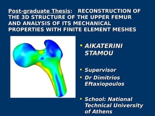
1. Post-graduate ThesisPost-graduate Thesis: RECONSTRUCTION OF: RECONSTRUCTION OF
THE 3D STRUCTURE OF THE UPPER FEMURTHE 3D STRUCTURE OF THE UPPER FEMUR
AND ANALYSIS OF ITS MECHANICALAND ANALYSIS OF ITS MECHANICAL
PROPERTIES WITH FINITE ELEMENT MESHESPROPERTIES WITH FINITE ELEMENT MESHES
• AIKATERINIAIKATERINI
STAMOUSTAMOU
• SupervisorSupervisor
• DrDr DimitriosDimitrios
EftaxiopoulosEftaxiopoulos
• School: NationalSchool: National
Technical UniversityTechnical University
of Athensof Athens

2. Objectives of the workObjectives of the work
• Reconstruction of the human upper femur fromReconstruction of the human upper femur from
computational tomography imagescomputational tomography images
• Modeling its mechanics withModeling its mechanics with finite elementsfinite elements

3. 1.1.Introduction to BiomechanicsIntroduction to Biomechanics
2.2.Anatomy of the upper femurAnatomy of the upper femur
3.3.Segmentation of the computational tomographySegmentation of the computational tomography
images with algorithms of the software bookcaseimages with algorithms of the software bookcase
Insight Toolkit (ITK)Insight Toolkit (ITK)
4.4.Modeling and discretization of the upper femurModeling and discretization of the upper femur
Creation of the composite boneCreation of the composite bone
5.5.Solving differential equations in the discretized femurSolving differential equations in the discretized femur
bone Specially, solving Navier-Stokes equations inbone Specially, solving Navier-Stokes equations in
the bone which accepts static loadingthe bone which accepts static loading
6.6.ConclusionsConclusions
ContentsContents

4. 1.1. Introduction to BiomechanicsIntroduction to Biomechanics
 Galileo (1638)Galileo (1638) Studied the mechanics of long bones andStudied the mechanics of long bones and
analyzed the gross anatomical structure of the thighanalyzed the gross anatomical structure of the thigh
 WolfWolf (1870) The structures were found not to be irregular in(1870) The structures were found not to be irregular in
orientation, but aligned to form a sophisticated patternorientation, but aligned to form a sophisticated pattern
 (1892) The bone structures were not only predetermined by(1892) The bone structures were not only predetermined by
genetic factors but also by adaptation to mechanical loadgenetic factors but also by adaptation to mechanical load
situationsituation
 Koch (1917)Koch (1917) First tried to quantify the mechanical situationFirst tried to quantify the mechanical situation
within the femur by calculating the stresses and strainswithin the femur by calculating the stresses and strains
 Torodls (1969)Torodls (1969) The effect of the muscle loads on theThe effect of the muscle loads on the
mechanical behavior of the femur was not as important asmechanical behavior of the femur was not as important as
that of the body weightthat of the body weight
 Ghista (1976)Ghista (1976) A complete mathematical description of theA complete mathematical description of the
internal stresses in a leg during gaitinternal stresses in a leg during gait

5. 2. Anatomy of the upper femur2. Anatomy of the upper femur
 The head:The head: The head which isThe head which is
globular and forms rather moreglobular and forms rather more
than a hemisphere Its surface isthan a hemisphere Its surface is
smooth, coated with cartilage insmooth, coated with cartilage in
the fresh state, except over anthe fresh state, except over an
ovoid depression, the fovea capitisovoid depression, the fovea capitis
femoris, which is situated a littlefemoris, which is situated a little
below and behind the center of thebelow and behind the center of the
headhead
 The neck:The neck: In addition toIn addition to
projecting upward and medialwardprojecting upward and medialward
from the body of the femur, thefrom the body of the femur, the
neck projects forward; the amountneck projects forward; the amount
of thof thee forward projection isforward projection is
extremely variable, but on anextremely variable, but on an
average is from 12° to 14°.average is from 12° to 14°.
 The greater trochanter:The greater trochanter: AA large,large,
irregular, quadrilateral eminence,irregular, quadrilateral eminence,
situated at the junction of the necksituated at the junction of the neck
with the upper part of the bodywith the upper part of the body
 The lesser trochanter:The lesser trochanter: AA
conical eminence, which projectsconical eminence, which projects
from the lower and back part of thefrom the lower and back part of the
base of the neck.base of the neck.

6. 3.3. Insight Toolkit (ITK)Insight Toolkit (ITK) applicationsapplications
• Segmentation: the process of identifying andSegmentation: the process of identifying and
classifying data found in a digitally samplingclassifying data found in a digitally sampling
representationrepresentation
• The basic approach of a region growing algorithm isThe basic approach of a region growing algorithm is
to start from a seed region (typically one or moreto start from a seed region (typically one or more
pixels) that are considered to be inside the object topixels) that are considered to be inside the object to
be segmented. The pixels neighboringbe segmented. The pixels neighboring
this region are evaluated to determine if they shouldthis region are evaluated to determine if they should
also be considered part of the object. If so, they arealso be considered part of the object. If so, they are
added to the region and the process continues as longadded to the region and the process continues as long
as new pixels are added toas new pixels are added to
the region.the region.
Region growing algorithms vary dependent on theRegion growing algorithms vary dependent on the
criteria:criteria:
• A) a pixel should be included in the regionA) a pixel should be included in the region
• B) the type connectivity used to determine neighborsB) the type connectivity used to determine neighbors
• C) the strategy used to visit neighboring pixelsC) the strategy used to visit neighboring pixels

7. Connected Threshold algorithmConnected Threshold algorithm
• A simple criterion for includingA simple criterion for including
pixels in a growing region is topixels in a growing region is to
evaluate intensity value insideevaluate intensity value inside
a specific interval.a specific interval.
• Most of the algorithmic complexity ofMost of the algorithmic complexity of
a region growing method comes froma region growing method comes from
visiting neighboring pixels.visiting neighboring pixels.
• The algorithm is left to establish aThe algorithm is left to establish a
criterion to decide whether acriterion to decide whether a
particular pixel should be included inparticular pixel should be included in
the current region.the current region.
• The criterion used by theThe criterion used by the
ConnectedThresholdImageFilter is basedConnectedThresholdImageFilter is based
on an interval of intensity values providedon an interval of intensity values provided
by the user. Values of lower and upperby the user. Values of lower and upper
threshold should be provided. The regionthreshold should be provided. The region
growing algorithm includes those pixelsgrowing algorithm includes those pixels
whose intensities are inside the interval.whose intensities are inside the interval.
∈l(x) [lower,upper]l(x) [lower,upper]

8. Confidence-Connected algorithmConfidence-Connected algorithm
• The criterion used is based on simpleThe criterion used is based on simple
statistics of the current region.statistics of the current region.
• First, the algorithm computes the mean andFirst, the algorithm computes the mean and
standard deviation of intensity values for all thestandard deviation of intensity values for all the
pixels currently included in the region.pixels currently included in the region.
• A user-provided factor is used to multiply theA user-provided factor is used to multiply the
standard deviation and define a range aroundstandard deviation and define a range around
the mean. Neighbor pixels whose intensitythe mean. Neighbor pixels whose intensity
values fall inside the range are accepted andvalues fall inside the range are accepted and
included in the region. When no moreincluded in the region. When no more
neighboring pixels are found that satisfy theneighboring pixels are found that satisfy the
criterion, the algorithm is considered to havecriterion, the algorithm is considered to have
finished its first iteration.finished its first iteration.
• Then, the mean and standard deviation of theThen, the mean and standard deviation of the
intensity levels are recomputed using all theintensity levels are recomputed using all the
pixels currently included in the region. Thispixels currently included in the region. This
mean and standard deviation defines anewmean and standard deviation defines anew
intensity range that is used to visit currentintensity range that is used to visit current
region neighbors and evaluate whether theirregion neighbors and evaluate whether their
intensity falls inside the range.intensity falls inside the range.
( ) [ ]σσ fm,fmXl +−∈

9. 4.4. SoftwareSoftware SlicerSlicer and segmentation methodand segmentation method
• It is used for the imaging and processing of MRI forIt is used for the imaging and processing of MRI for
the discretisation of the bone. Image DICOM isthe discretisation of the bone. Image DICOM is
processed from a segmentation with the simple regionprocessed from a segmentation with the simple region
growing method.growing method.
• Simple region growing method is described from aSimple region growing method is described from a
statistic segmentation algorithm.statistic segmentation algorithm.
• The algorithm uses seeds as data.The algorithm uses seeds as data.
• The algorithm computes the mean and standardThe algorithm computes the mean and standard
deviation of intensity values for all the pixelsdeviation of intensity values for all the pixels
currently included in the seed region. Using thecurrently included in the seed region. Using the
standard deviation as a radius, the region extendsstandard deviation as a radius, the region extends
and the pixels with intensity which belongsand the pixels with intensity which belongs
in the interval (range) are located (found) there.in the interval (range) are located (found) there.

10. Imaging the tomography in SlicerImaging the tomography in Slicer

11. Views of tomography in SlicerViews of tomography in Slicer

12. Creation of the volume of the marrow cavityCreation of the volume of the marrow cavity
with automated segmentationwith automated segmentation

13. Volume models of the marrow cavityVolume models of the marrow cavity
• Model without smoothingModel without smoothing
• Model with big smoothingModel with big smoothing
100smooth =

14. Creation of the cancellous bone usingCreation of the cancellous bone using
module Editormodule Editor
• Label mapLabel map ofof
the marrowthe marrow
cavitycavity
• Result of EditorResult of Editor
on theon the
cancellous bonecancellous bone
((anterior-anterior-
posteriorposterior))

15. Creation of the composite bone usingCreation of the composite bone using
module Editormodule Editor

16. Volume modelVolume model of cancellous boneof cancellous bone
(Number of Iterations: 50, Decimate: 0.05)

17. Volume model of cortical boneVolume model of cortical bone
(Number of Iterations:50, Decimate: 0.05)

18. Discretisation of the bone from the software GmshDiscretisation of the bone from the software Gmsh
• Gmsh is an automatic three-dimensional finiteGmsh is an automatic three-dimensional finite
element mesh generator with built-in pre- andelement mesh generator with built-in pre- and
post-processing facilities. Its design goal is topost-processing facilities. Its design goal is to
provide a simple meshing tool for academicprovide a simple meshing tool for academic
problems.problems.
Main characteristics ofMain characteristics of GmshGmsh
• QQuickly describe simple and/or “repetitive” geometries,uickly describe simple and/or “repetitive” geometries,
thanks to user-defined functions,thanks to user-defined functions, loops, conditionalsloops, conditionals..
PParametrize these geometries.arametrize these geometries.
• GGenerate 1D, 2D and 3D simplicialenerate 1D, 2D and 3D simplicial finite element meshesfinite element meshes
• CCreate simple extruded geometries and meshesreate simple extruded geometries and meshes
• GGenerate complex animationsenerate complex animations
• VVisualize computational results in a great variety ofisualize computational results in a great variety of
ways. Gmsh can display scalar,vector and tensorways. Gmsh can display scalar,vector and tensor
datasets, and can perform various operations on thedatasets, and can perform various operations on the
resulting postprocessingresulting postprocessing viewsviews..

19. Meshing of surfaces and volumes on GmshMeshing of surfaces and volumes on Gmsh
Cancellous Bone

20. Clipping of the discretised cancellous boneClipping of the discretised cancellous bone

21. ChoiceChoice StatisticsStatistics ofof GmshGmsh for the compositefor the composite
bonebone
• The frame model volumeThe frame model volume
of the discretizedof the discretized
composite bonecomposite bone
incorporatesincorporates
106888 Triangles106888 Triangles
397552 Tetrahedra397552 Tetrahedra

22. SurfacesSurfaces of the discretised compositeof the discretised composite
bonebone

23. Clipping of the discretised composite boneClipping of the discretised composite bone
• Inside from the choiceInside from the choice ToolsTools→→Clipping PlanesClipping Planes withwith
the choicethe choice Clipping PlaneClipping Plane 44 we can take thewe can take the
upper imageupper image..
• Volumes of bone undertaking clipping are imagedVolumes of bone undertaking clipping are imaged
upper.upper.
Clippingplane 4

24. Discretized composite bone with definedDiscretized composite bone with defined
surfaces of zero degrees of freedom (DOF)surfaces of zero degrees of freedom (DOF)

25. 5.5. The softwareThe software FreeFem++FreeFem++
 The FreeFem++The FreeFem++
• Problem description (real or complex valued) by theirProblem description (real or complex valued) by their
variational formulations, with access to the internalvariational formulations, with access to the internal
vectors and matrices if needed.vectors and matrices if needed.
• Multi-variables, multi-equations, bi-dimensional , staticMulti-variables, multi-equations, bi-dimensional , static
or time dependent, linear or nonlinear coupledor time dependent, linear or nonlinear coupled
systems; however the user is required to describe thesystems; however the user is required to describe the
iterative procedures which reduce the problem to a setiterative procedures which reduce the problem to a set
of linear problems.of linear problems.
• High level user friendly typed input language with anHigh level user friendly typed input language with an
algebra of analytic and finite element functions.algebra of analytic and finite element functions.
• A large variety of triangular finite elements : linearA large variety of triangular finite elements : linear
and quadratic Lagrangian elements, discontinuous P1and quadratic Lagrangian elements, discontinuous P1
and Raviart-Thomasand Raviart-Thomas
elements, elements of a non-scalar type, mini-elementelements, elements of a non-scalar type, mini-element
(but no quadrangles).(but no quadrangles).

26. Creation of the composite boneCreation of the composite bone
• CodeCode getmeshgetmesh..edpedp
mesh3 Th1("floioskat.mesh");mesh3 Th1("floioskat.mesh");
mesh3 Th2("spogkat.mesh");mesh3 Th2("spogkat.mesh");
int[int] r1=[3,5], r2=[1,7];int[int] r1=[3,5], r2=[1,7];
mesh3mesh3 Th3=tetgreconstructionTh3=tetgreconstruction (Th2,(Th2, switchswitch
="rYYCVVV",refface=r2,="rYYCVVV",refface=r2,
reftet=r1);reftet=r1);
mesh3 Th=Th1+Th3;mesh3 Th=Th1+Th3;

27. Solving equations of Elasticity with the effect ofSolving equations of Elasticity with the effect of
gravitygravity
Variation formulationVariation formulation
PutPut andand zerozero
displacementdisplacement
exterior to the compositeexterior to the composite
bonebone
solvesolve Elasticity([u1,u2,u3],Elasticity([u1,u2,u3],
[v1,v2,v3],solver=CG)=int3d(T[v1,v2,v3],solver=CG)=int3d(T
h)h)
((Ep*nu/((1.+nu)*(1.-2.*nu)))((Ep*nu/((1.+nu)*(1.-2.*nu)))
*div(u1,u2,u3) *div(v1,v2,v3)*div(u1,u2,u3) *div(v1,v2,v3)
( ) ( )
( ) ( ) ( )( ) ( )( )
( ) ( ) 0vfdxdxv:u2v.u.
vuv:u
0vfdxdxv:u
j,i
ijij
=−+∇∇








=
=−
∫∫
∑
∫∫
ΩΩ
ΩΩ
εµελ
εσεσ
εσ
1f =
SolutionSolution u2u2

28. SolvingSolving NavierNavier equations on the human upper femurequations on the human upper femur
during walkingduring walking
Ph reg=region, Ep, nu;Ph reg=region, Ep, nu;
int floios=reg(-141.642, -11.5074, 6.68015);int floios=reg(-141.642, -11.5074, 6.68015);
Ep=600.+17000.*(region==floios);Ep=600.+17000.*(region==floios);
nu=0.3-0.02*(region==floios);nu=0.3-0.02*(region==floios);
Region functionRegion function

29. Young’s modulusYoung’s modulus

30. real volume55= int3d(Th,55)(1.);real volume55= int3d(Th,55)(1.);
real area70= int2d(Th,70)(1.);real area70= int2d(Th,70)(1.);
real area115= int2d(Th,115)(1.);real area115= int2d(Th,115)(1.);
real area190= int2d(Th,190)(1.);real area190= int2d(Th,190)(1.);
solve Elasticity([u1,u2,u3],[v1,v2,v3],solver=CG)=solve Elasticity([u1,u2,u3],[v1,v2,v3],solver=CG)=
int3d(Th)((Ep*nu/((1.+nu)*(1.-2.*nu)))*div(u1,u2,u3)*div(v1,v2,v3)int3d(Th)((Ep*nu/((1.+nu)*(1.-2.*nu)))*div(u1,u2,u3)*div(v1,v2,v3)
+2.*(Ep/(2.*(1.+nu)))*(epsilon(u1,u2,u3)'*epsilon(v1,v2,v3)))+2.*(Ep/(2.*(1.+nu)))*(epsilon(u1,u2,u3)'*epsilon(v1,v2,v3)))
-int3d(Th,55)(((-0.54/volume55)*836)*v1)-int3d(Th,55)(((-0.54/volume55)*836)*v1)
-int3d(Th,55)(((-0.328/volume55)*836)*v2)-int3d(Th,55)(((-0.328/volume55)*836)*v2)
-int3d(Th,55)(((-2.292/volume55)*836)*v3)-int3d(Th,55)(((-2.292/volume55)*836)*v3)
-int3d(Th,55)(((-0.081/volume55)*836)*v1)-int3d(Th,55)(((-0.081/volume55)*836)*v1)
-int3d(Th,55)(((-0.128/volume55)*836)*v2)-int3d(Th,55)(((-0.128/volume55)*836)*v2)
-int3d(Th,55)(((-0.782/volume55)*836)*v3)-int3d(Th,55)(((-0.782/volume55)*836)*v3)
-int2d(Th,70)(((0.58/area70)*836)*v1)-int2d(Th,70)(((0.58/area70)*836)*v1)
-int2d(Th,70)(((0.043/area70)*836)*v2)-int2d(Th,70)(((0.043/area70)*836)*v2)
-int2d(Th,70)(((0.865/area70)*836)*v3)-int2d(Th,70)(((0.865/area70)*836)*v3)
-int2d(Th,70)(((0.072/area70)*836)*v1)-int2d(Th,70)(((0.072/area70)*836)*v1)
-int2d(Th,70)(((0.116/area70)*836)*v2)-int2d(Th,70)(((0.116/area70)*836)*v2)
-int2d(Th,70)(((0.132/area70)*836)*v3)-int2d(Th,70)(((0.132/area70)*836)*v3)
-int2d(Th,70)(((-0.005/area70)*836)*v1)-int2d(Th,70)(((-0.005/area70)*836)*v1)
-int2d(Th,70)(((-0.007/area70)*836)*v2)-int2d(Th,70)(((-0.007/area70)*836)*v2)
-int2d(Th,70)(((-0.19/area70)*836)*v3)-int2d(Th,70)(((-0.19/area70)*836)*v3)
-int2d(Th,190)(((-0.009/area190)*836)*v1)-int2d(Th,190)(((-0.009/area190)*836)*v1)
-int2d(Th,190)(((0.185/area190)*836)*v2)-int2d(Th,190)(((0.185/area190)*836)*v2)
-int2d(Th,190)(((-0.929/area190)*836)*v3)-int2d(Th,190)(((-0.929/area190)*836)*v3)
+on(19,u1=0,u2=0,u3=0) +on(16,u1=0,u2=0,u3=0);+on(19,u1=0,u2=0,u3=0) +on(16,u1=0,u2=0,u3=0);

31. Norm of the displacementNorm of the displacement
• The maximum value is appeared in the headThe maximum value is appeared in the head and the zeroand the zero
value in the surfaces with zero Degrees of Freedomvalue in the surfaces with zero Degrees of Freedom..

32. First principal strainFirst principal strain
Big strains in the neck
The neck is characterized as a bending bar with tension in the upper
part.
The upper part of the neck is a possible point of beginning the fracture
because the bending cortical is very thin.

33. • Big strains between theBig strains between the
loading surfaces.loading surfaces.
It is due to the big tensionIt is due to the big tension
which loads create locally,which loads create locally,
but also the bending of thebut also the bending of the
diaphysis, which has thediaphysis, which has the
tensile region outsidetensile region outside
because of the press ofbecause of the press of
pelvis to the head.pelvis to the head.
• Big strains in the smallBig strains in the small
loading surfaces due to theloading surfaces due to the
small concentration ofsmall concentration of
strains as a result of beingstrains as a result of being
the small loading surfaces.the small loading surfaces.

34. MaximumMaximum shearshear strainstrain
• Maximum values in the upper neck and exterior toMaximum values in the upper neck and exterior to
the diaphysis.the diaphysis.
• Possible failure due to shear is assumed on thesePossible failure due to shear is assumed on these
regions.regions.

35. MinimumMinimum principal strainprincipal strain
• The maximum compression is developed in theThe maximum compression is developed in the
lower neck and interior to the diaphysis.lower neck and interior to the diaphysis.

36. Maximum shear stressMaximum shear stress
• Big shear strains are developed exterior to theBig shear strains are developed exterior to the
diaphysis, around the muscle loading regions anddiaphysis, around the muscle loading regions and
interior to the diaphysis.interior to the diaphysis.

37. Strain energyStrain energy
• Maximum strain energy is developed interior toMaximum strain energy is developed interior to
the diaphysis and in the lower neck.the diaphysis and in the lower neck.

38. Solving Navier-Stokes equations in theSolving Navier-Stokes equations in the
human upper femurhuman upper femur
during stair-climbingduring stair-climbing
solve Elasticity([u1,u2,u3],[v1,v2,v3],solver=CG)=solve Elasticity([u1,u2,u3],[v1,v2,v3],solver=CG)=int3d(Th)int3d(Th)
((Ep*nu/((1.+nu)((Ep*nu/((1.+nu)**
(1.-2.*nu))*div(u1,u2,u3)*div(v1,v2,v3)+2.*(Ep/(1.-2.*nu))*div(u1,u2,u3)*div(v1,v2,v3)+2.*(Ep/
(2.*(1.+nu)))*(epsilon(u1,u2,u3)(2.*(1.+nu)))*(epsilon(u1,u2,u3)
'' *epsilon(v1,v2,v3)))*epsilon(v1,v2,v3)))
-int3d(Th,55)(((-0.593/volume55)*847)*v1)-int3d(Th,55)(((-0.593/volume55)*847)*v1)
........................................................................................................................................................................................................
..................................
........................................................................................................................................................................................................
................................
-int2d(Th,115)(((-0.088/area115)*847)*v1)-int2d(Th,115)(((-0.088/area115)*847)*v1)
-int2d(Th,115)(((0.396/area115)*847)*v2)-int2d(Th,115)(((0.396/area115)*847)*v2)
-int2d(Th,115)(((-2.671/area115)*847)*v3)-int2d(Th,115)(((-2.671/area115)*847)*v3) ;;
+on(19,u1=0,u2=0,u3=0)+on(19,u1=0,u2=0,u3=0)
+on(16,u1=0,u2=0,u3=0);+on(16,u1=0,u2=0,u3=0);

39. Displacement in the direction of the x-axisDisplacement in the direction of the x-axis
• Zero values in the surfaces with zero Degrees ofZero values in the surfaces with zero Degrees of
Freedom.Freedom.
• Maximum x-displacement in the neck, where theMaximum x-displacement in the neck, where the
maximum load is implemented.maximum load is implemented.

40. Maximum principal strainMaximum principal strain
• Big strains interior and exterior to the diaphysis, also in theBig strains interior and exterior to the diaphysis, also in the
upper and lower neck and in the conjunction of the neckupper and lower neck and in the conjunction of the neck
and the head.and the head.

41. Maximum shear strainMaximum shear strain
• Big strains are developed in the lower part of the neckBig strains are developed in the lower part of the neck
and interior to the diaphysis.and interior to the diaphysis.

42. Minimum principal strainMinimum principal strain
• Maximum compression is developed in the lower part of theMaximum compression is developed in the lower part of the
neck and interior to the diaphysis.neck and interior to the diaphysis.

43. Von Misses stressVon Misses stress
• Bigger stresses are developed interior to the diaphysisBigger stresses are developed interior to the diaphysis..

44. Strain energyStrain energy
• Maximum strain energy is developed interior to theMaximum strain energy is developed interior to the
diaphysis.diaphysis.

45. 6.6. ConclusionsConclusions
➢WalkingWalking

The bigger tension is developed in the cortical bone, exterior toThe bigger tension is developed in the cortical bone, exterior to
the diaphysis and in the upper part of the neck. The possibilitythe diaphysis and in the upper part of the neck. The possibility
of beginning the failure is bigger there, because the corticalof beginning the failure is bigger there, because the cortical
bone is brittle and it appears small tolerance in tension.bone is brittle and it appears small tolerance in tension.
Maximum shear is developed there.Maximum shear is developed there.

The bigger compression is developed interior to the diaphysisThe bigger compression is developed interior to the diaphysis
and in the lower part of the neck, in the cortical bone. Theand in the lower part of the neck, in the cortical bone. The
cortical bone appears big tolerance in compression. There is thecortical bone appears big tolerance in compression. There is the
danger of failure due to compression interior to the diaphysisdanger of failure due to compression interior to the diaphysis
and in the lower part of the neck because of pathologicaland in the lower part of the neck because of pathological
situations.situations.

The Von Misses stress and strain energy density are maximumThe Von Misses stress and strain energy density are maximum
interior to the diaphysis and in the lower part of the neck, in theinterior to the diaphysis and in the lower part of the neck, in the
cortical bone due to big compression there.cortical bone due to big compression there.
➢Stair-climbingStair-climbing
●
Similar notes with those of walkingSimilar notes with those of walking
●
Only quantified differences between walking and stair-climbingOnly quantified differences between walking and stair-climbing
●
No qualified differences between walking and stair-climbingNo qualified differences between walking and stair-climbing

46. ReferencesReferences
 Gray’s anatomyGray’s anatomy
Henry Gray (1821-1865)Henry Gray (1821-1865)
Anatomy of the human bodyAnatomy of the human body
 Determination of muscle loading at the hip joint for use in pre-Determination of muscle loading at the hip joint for use in pre-
clinical testingclinical testing
M.O. Heller, G. Bergmann, J.-P. Kassi, L. Claes, N.P. Haas, G.N.M.O. Heller, G. Bergmann, J.-P. Kassi, L. Claes, N.P. Haas, G.N.
DudaDuda
Magazine: Journal of Biomechanics 38 (2005)Magazine: Journal of Biomechanics 38 (2005)
1155–11631155–1163
 FreeFem++ (2009FreeFem++ (2009))
 Gmsh (2009)Gmsh (2009)
 ITK (Insight Segmentation and Registration Toolkit, 2009)ITK (Insight Segmentation and Registration Toolkit, 2009)
 Medit (2009)Medit (2009)
 Slicer (2009)Slicer (2009)
 Tetgen (2009)Tetgen (2009)
 Visible Human Project (2009)Visible Human Project (2009)