SlideShare une entreprise Scribd logo
1  sur  122
Télécharger pour lire hors ligne
1/43
Intrusion Response through Optimal Stopping
New York University - Invited Talk
Kim Hammar
kimham@kth.se
Division of Network and Systems Engineering
KTH Royal Institute of Technology
Intrusion event
time-step t = 1 Intrusion ongoing
t
t = T
Early stopping times Stopping times that
affect the intrusion
Episode
2/43
Use Case: Intrusion Response
I A Defender owns an infrastructure
I Consists of connected components
I Components run network services
I Defender defends the infrastructure
by monitoring and active defense
I Has partial observability
I An Attacker seeks to intrude on the
infrastructure
I Has a partial view of the
infrastructure
I Wants to compromise specific
components
I Attacks by reconnaissance,
exploitation and pivoting
Attacker Clients
. . .
Defender
1 IPS
1
alerts
Gateway
7 8 9 10 11
6
5
4
3
2
12
13 14 15 16
17
18
19
21
23
20
22
24
25 26
27 28 29 30 31
3/43
Intrusion Response from the Defender’s Perspective
20 40 60 80 100 120 140 160 180 200
0.5
1
t
b
20 40 60 80 100 120 140 160 180 200
50
100
150
200
t
Alerts
20 40 60 80 100 120 140 160 180 200
5
10
15
t
Logins
3/43
Intrusion Response from the Defender’s Perspective
20 40 60 80 100 120 140 160 180 200
0.5
1
t
b
20 40 60 80 100 120 140 160 180 200
50
100
150
200
t
Alerts
20 40 60 80 100 120 140 160 180 200
5
10
15
t
Logins
3/43
Intrusion Response from the Defender’s Perspective
20 40 60 80 100 120 140 160 180 200
0.5
1
t
b
20 40 60 80 100 120 140 160 180 200
50
100
150
200
t
Alerts
20 40 60 80 100 120 140 160 180 200
5
10
15
t
Logins
3/43
Intrusion Response from the Defender’s Perspective
20 40 60 80 100 120 140 160 180 200
0.5
1
t
b
20 40 60 80 100 120 140 160 180 200
50
100
150
200
t
Alerts
20 40 60 80 100 120 140 160 180 200
5
10
15
t
Logins
3/43
Intrusion Response from the Defender’s Perspective
20 40 60 80 100 120 140 160 180 200
0.5
1
t
b
20 40 60 80 100 120 140 160 180 200
50
100
150
200
t
Alerts
20 40 60 80 100 120 140 160 180 200
5
10
15
t
Logins
3/43
Intrusion Response from the Defender’s Perspective
20 40 60 80 100 120 140 160 180 200
0.5
1
t
b
20 40 60 80 100 120 140 160 180 200
50
100
150
200
t
Alerts
20 40 60 80 100 120 140 160 180 200
5
10
15
t
Logins
3/43
Intrusion Response from the Defender’s Perspective
20 40 60 80 100 120 140 160 180 200
0.5
1
t
b
20 40 60 80 100 120 140 160 180 200
50
100
150
200
t
Alerts
20 40 60 80 100 120 140 160 180 200
5
10
15
t
Logins
3/43
Intrusion Response from the Defender’s Perspective
20 40 60 80 100 120 140 160 180 200
0.5
1
t
b
20 40 60 80 100 120 140 160 180 200
50
100
150
200
t
Alerts
20 40 60 80 100 120 140 160 180 200
5
10
15
t
Logins
3/43
Intrusion Response from the Defender’s Perspective
20 40 60 80 100 120 140 160 180 200
0.5
1
t
b
20 40 60 80 100 120 140 160 180 200
50
100
150
200
t
Alerts
20 40 60 80 100 120 140 160 180 200
5
10
15
t
Logins
When to take a defensive action?
Which action to take?
4/43
Formulating Intrusion Response as a Stopping Problem
time-step t = 1
t
t = T
Episode
Attacker Clients
. . .
Defender
1 IDS
1
alerts
Gateway
7 8 9 10 11
6
5
4
3
2
12
13 14 15 16
17
18
19
21
23
20
22
24
25 26
27 28 29 30 31
I The system evolves in discrete time-steps.
I Defender observes the infrastructure (IDS, log files, etc.).
I An intrusion occurs at an unknown time.
I The defender can make L stops.
I Each stop is associated with a defensive action
I The final stop shuts down the infrastructure.
I Based on the observations, when is it optimal to stop?
4/43
Formulating Intrusion Response as a Stopping Problem
Intrusion event
time-step t = 1 Intrusion ongoing
t
t = T
Early stopping times Stopping times that
affect the intrusion
Episode
Attacker Clients
. . .
Defender
1 IDS
1
alerts
Gateway
7 8 9 10 11
6
5
4
3
2
12
13 14 15 16
17
18
19
21
23
20
22
24
25 26
27 28 29 30 31
I The system evolves in discrete time-steps.
I Defender observes the infrastructure (IDS, log files, etc.).
I An intrusion occurs at an unknown time.
I The defender can make L stops.
I Each stop is associated with a defensive action
I The final stop shuts down the infrastructure.
I Based on the observations, when is it optimal to stop?
5/43
Formulating Network Intrusion as a Stopping Problem
Intrusion event
(1st stop)
time-step t = 1 Intrusion ongoing
t
(2nd stop)
t = T
Episode
Attacker Clients
. . .
Defender
1 IDS
1
alerts
Gateway
7 8 9 10 11
6
5
4
3
2
12
13 14 15 16
17
18
19
21
23
20
22
24
25 26
27 28 29 30 31
I The system evolves in discrete time-steps.
I The attacker observes the infrastructure (IDS, log files, etc.).
I The first stop action decides when to intrude.
I The attacker can make 2 stops.
I The second stop action terminates the intrusion.
I Based on the observations & the defender’s belief, when
is it optimal to stop?
6/43
A Dynkin Game Between the Defender and the Attacker1
Attacker
Defender
t = 1
t = T
τ1,1 τ1,2 τ1,3
τ2,1
t
Stopped
Game episode
Intrusion
I We formalize the Dynkin game as a zero-sum partially
observed one-sided stochastic game.
I The defender is the maximizing player
I The attacker is the minimizing player
1
E.B Dynkin. “A game-theoretic version of an optimal stopping problem”. In: Dokl. Akad. Nauk SSSR 385
(1969), pp. 16–19.
7/43
Our Approach for Solving the Dynkin Game
s1,1 s1,2 s1,3 . . . s1,n
s2,1 s2,2 s2,3 . . . s2,n
.
.
.
.
.
.
.
.
.
.
.
.
.
.
.
Emulation System
Target
Infrastructure
Model Creation &
System Identification
Strategy Mapping
π
Selective
Replication
Strategy
Implementation π
Simulation System
Reinforcement Learning &
Generalization
Strategy evaluation &
Model estimation
Automation &
Self-learning systems
8/43
Outline
I Use Case & Approach
I Use case: Intrusion response
I Approach: Optimal stopping
I Theoretical Background & Formal Model
I Optimal stopping problem definition
I Formulating the Dynkin game as a one-sided POSG
I Structure of π∗
I Stopping sets Sl are connected and nested, S1 is convex.
I Existence of multi-threshold best response strategies π̃1, π̃2.
I Efficient Algorithms for Learning π∗
I T-SPSA: A stochastic approximation algorithm to learn π∗
I T-FP: A Fictitious-play algorithm to approximate (π∗
1 , π∗
2 )
I Evaluation Results
I Target system, digital twin, system identification, & results
I Conclusions & Future Work
9/43
Optimal Stopping: A Brief History
I History:
I Studied in the 18th century to analyze a gambler’s fortune
I Formalized by Abraham Wald in 19472
I Since then it has been generalized and developed by (Chow3
,
Shiryaev & Kolmogorov4
, Bather5
, Bertsekas6
, etc.)
2
Abraham Wald. Sequential Analysis. Wiley and Sons, New York, 1947.
3
Y. Chow, H. Robbins, and D. Siegmund. “Great expectations: The theory of optimal stopping”. In: 1971.
4
Albert N. Shirayev. Optimal Stopping Rules. Reprint of russian edition from 1969. Springer-Verlag Berlin,
2007.
5
John Bather. Decision Theory: An Introduction to Dynamic Programming and Sequential Decisions. USA:
John Wiley and Sons, Inc., 2000. isbn: 0471976490.
6
Dimitri P. Bertsekas. Dynamic Programming and Optimal Control. 3rd. Vol. I. Belmont, MA, USA: Athena
Scientific, 2005.
10/43
The Optimal Stopping Problem
I The General Problem:
I A stochastic process (st)T
t=1 is observed sequentially
I Two options per t: (i) continue to observe; or (ii) stop
I Find the optimal stopping time τ∗
:
τ∗
= arg max
τ
Eτ
" τ−1
X
t=1
γt−1
RC
st st+1
+ γτ−1
RS
sτ sτ
#
(1)
where RS
ss0 & RC
ss0 are the stop/continue rewards
I The L − lth stopping time τl is:
τl = inf{t : t > τl−1, at = S}, l ∈ 1, .., L, τL+1 = 0
I τl is a random variable from sample space Ω to N, which is
dependent on hτ = ρ1, a1, o1, . . . , aτ−1, oτ and independent of
aτ , oτ+1, . . .
I We consider the class of stopping times Tt = {τ ≤ t} ∈ Fk
where Fk is the natural filtration on ht.
I Solution approaches: the Markovian approach and the
martingale approach.
10/43
The Optimal Stopping Problem
I The General Problem:
I A stochastic process (st)T
t=1 is observed sequentially
I Two options per t: (i) continue to observe; or (ii) stop
I Find the optimal stopping time τ∗
:
τ∗
= arg max
τ
Eτ
" τ−1
X
t=1
γt−1
RC
st st+1
+ γτ−1
RS
sτ sτ
#
(2)
where RS
ss0 & RC
ss0 are the stop/continue rewards
I The L − lth stopping time τl is:
τl = inf{t : t > τl−1, at = S}, l ∈ 1, .., L, τL+1 = 0
I τl is a random variable from sample space Ω to N, which is
dependent on hτ = ρ1, a1, o1, . . . , aτ−1, oτ and independent of
aτ , oτ+1, . . .
I We consider the class of stopping times Tt = {τ ≤ t} ∈ Fk
where Fk is the natural filtration on ht.
I Solution approaches: the Markovian approach and the
martingale approach.
10/43
Optimal Stopping: Solution Approaches
I The Markovian approach:
I Model the problem as a MDP or POMDP
I A policy π∗
that satisfies the Bellman-Wald equation is
optimal:
π∗
(s) = arg max
{S,C}
"
E

RS
s

| {z }
stop
, E

RC
s + γV ∗
(s0
)

| {z }
continue
#
∀s ∈ S
I Solve by backward induction, dynamic programming, or
reinforcement learning
10/43
Optimal Stopping: Solution Approaches
I The Markovian approach:
I Assume all rewards are received upon stopping: R∅
s
I V ∗
(s) majorizes R∅
s if V ∗
(s) ≥ R∅
s ∀s ∈ S
I V ∗
(s) is excessive if V ∗
(s) ≥
P
s0 PC
s0sV ∗
(s0
) ∀s ∈ S
I V ∗
(s) is the minimal excessive function which majorizes R∅
s .
s
R∅
s
P
s0
PC
ss0 V ∗
(s0
)
V ∗
(s)
10/43
Optimal Stopping: Solution Approaches
I The martingale approach:
I Model the state process as an arbitrary stochastic process
I The reward of the optimal stopping time is given by the
smallest supermartingale that stochastically dominates the
process, called the Snell envelope7
.
7
J. L. Snell. “Applications of martingale system theorems”. In: Transactions of the American Mathematical
Society 73 (1952), pp. 293–312.
11/43
The Defender’s Optimal Stopping problem as a POMDP
I States:
I Intrusion state st ∈ {0, 1}, terminal ∅.
I Observations:
I IDS Alerts weighted by priority ot, stops
remaining lt ∈ {1, .., L}, f (ot|st)
I Actions:
I “Stop” (S) and “Continue” (C)
I Rewards:
I Reward: security and service. Penalty:
false alarms and intrusions
I Transition probabilities:
I Bernoulli process (Qt)T
t=1 ∼ Ber(p)
defines intrusion start It ∼ Ge(p)
I Objective and Horizon:
I max Eπ
hPT∅
t=1 r(st, at)
i
, T∅
0 1
∅
t ≥ 1
lt  0
t ≥ 2
lt  0
intrusion starts
Qt = 1
final stop
lt = 0
intrusion prevented
lt = 0
5 10 15 20 25
intrusion start time t
0.0
0.5
1.0
CDF
I
t
(t)
It ∼ Ge(p = 0.2)
12/43
The Attacker’s Optimal Stopping problem as an MDP
I States:
I Intrusion state st ∈ {0, 1}, terminal ∅,
defender belief b ∈ [0, 1].
I Actions:
I “Stop” (S) and “Continue” (C)
I Rewards:
I Reward: denial of service and intrusion.
Penalty: detection
I Transition probabilities:
I Intrusion starts and ends when the
attacker takes stop actions
I Objective and Horizon:
I max Eπ
hPT∅
t=1 r(st, at)
i
, T∅
0 1
∅
t ≥ 1 t ≥ 2
intrusion starts
at = 1
final stop detected
13/43
The Dynkin Game as a One-Sided POSG
I Players:
I Player 1 is the defender and player 2 is the
attacker. Hence, N = {1, 2}.
I Actions:
I A1 = A2 = {S, C}.
I Rewards:
I Zero-sum game. Defender maximizes, attacker
minimizes.
I Observability:
I The defender has partial observability. The
attacker has full observability.
I Obective functions:
J1(π1, π2) = E(π1,π2)
 T
X
t=1
γt−1
R(st, at)
#
(3)
J2(π1, π2) = −J1(π1, π2) (4)
0 1
∅
t ≥ 1
l  0
t ≥ 2
l  0
a
(2)
t = S
l
=
1
,
a
(
1
)
t
=
S
l
=
1
,
a
(
1
)
t
=
S
i
n
t
r
u
s
i
o
n
s
t
o
p
p
e
d
w
.
p
φ
l
o
r
t
e
r
m
i
n
a
t
e
d
(
a
(
2
)
t
=
S
)
14/43
Outline
I Use Case  Approach
I Use case: Intrusion response
I Approach: Optimal stopping
I Theoretical Background  Formal Model
I Optimal stopping problem definition
I Formulating the Dynkin game as a one-sided POSG
I Structure of π∗
I Stopping sets Sl are connected and nested, S1 is convex.
I Existence of multi-threshold best response strategies π̃1, π̃2.
I Efficient Algorithms for Learning π∗
I T-SPSA: A stochastic approximation algorithm to learn π∗
I T-FP: A Fictitious-play algorithm to approximate (π∗
1 , π∗
2 )
I Evaluation Results
I Target system, digital twin, system identification,  results
I Conclusions  Future Work
15/43
Structural Result: Optimal Multi-Threshold Policy
Theorem
Given the intrusion response POMDP, the following holds:
1. Sl−1 ⊆ Sl for l = 2, . . . L.
2. If L = 1, there exists an optimal threshold α∗ ∈ [0, 1] and an
optimal defender policy of the form:
π∗
L(b(1)) = S ⇐⇒ b(1) ≥ α∗
(5)
3. If L ≥ 1 and fX is totally positive of order 2 (TP2), there
exists L optimal thresholds α∗
l ∈ [0, 1] and an optimal
defender policy of the form:
π∗
l (b(1)) = S ⇐⇒ b(1) ≥ α∗
l , l = 1, . . . , L (6)
where α∗
l is decreasing in l.
15/43
Structural Result: Optimal Multi-Threshold Policy
Theorem
Given the intrusion response POMDP, the following holds:
1. Sl−1 ⊆ Sl for l = 2, . . . L.
2. If L = 1, there exists an optimal threshold α∗ ∈ [0, 1] and an
optimal defender policy of the form:
π∗
L(b(1)) = S ⇐⇒ b(1) ≥ α∗
(7)
3. If L ≥ 1 and fX is totally positive of order 2 (TP2), there
exists L optimal thresholds α∗
l ∈ [0, 1] and an optimal
defender policy of the form:
π∗
l (b(1)) = S ⇐⇒ b(1) ≥ α∗
l , l = 1, . . . , L (8)
where α∗
l is decreasing in l.
15/43
Structural Result: Optimal Multi-Threshold Policy
Theorem
Given the intrusion response POMDP, the following holds:
1. Sl−1 ⊆ Sl for l = 2, . . . L.
2. If L = 1, there exists an optimal threshold α∗ ∈ [0, 1] and an
optimal defender policy of the form:
π∗
L(b(1)) = S ⇐⇒ b(1) ≥ α∗
(9)
3. If L ≥ 1 and fX is totally positive of order 2 (TP2), there
exists L optimal thresholds α∗
l ∈ [0, 1] and an optimal
defender policy of the form:
π∗
l (b(1)) = S ⇐⇒ b(1) ≥ α∗
l , l = 1, . . . , L (10)
where α∗
l is decreasing in l.
15/43
Structural Result: Optimal Multi-Threshold Policy
Theorem
Given the intrusion response POMDP, the following holds:
1. Sl−1 ⊆ Sl for l = 2, . . . L.
2. If L = 1, there exists an optimal threshold α∗ ∈ [0, 1] and an
optimal defender policy of the form:
π∗
L(b(1)) = S ⇐⇒ b(1) ≥ α∗
(11)
3. If L ≥ 1 and fX is totally positive of order 2 (TP2), there
exists L optimal thresholds α∗
l ∈ [0, 1] and an optimal
defender policy of the form:
π∗
l (b(1)) = S ⇐⇒ b(1) ≥ α∗
l , l = 1, . . . , L (12)
where α∗
l is decreasing in l.
16/43
Structural Result: Optimal Multi-Threshold Policy
b(1)
0 1
belief space B = [0, 1]
16/43
Structural Result: Optimal Multi-Threshold Policy
b(1)
0 1
belief space B = [0, 1]
S1
α∗
1
16/43
Structural Result: Optimal Multi-Threshold Policy
b(1)
0 1
belief space B = [0, 1]
S1
S2
α∗
1
α∗
2
16/43
Structural Result: Optimal Multi-Threshold Policy
b(1)
0 1
belief space B = [0, 1]
S1
S2
.
.
.
SL
α∗
1
α∗
2
α∗
L
. . .
17/43
Lemma: V ∗
(b) is Piece-wise Linear and Convex
Lemma
V ∗(b) is piece-wise linear and convex.
I Belief space B is the |S − 1| dimensional unit simplex.
I |B| = ∞, high-dimensional (|S − 1|) continuous vector
I Infinite set of deterministic policies: maxπ:B→A Eπ
 P
t rt

B(3): 2-dimensional unit-simplex
0.25 0.55
0.2
(1, 0, 0) (0, 1, 0)
(0, 0, 1)
(0.25, 0.55, 0.2)
B(2): 1-dimensional unit-simplex
(1, 0) (0, 1)
0.4 0.6
(0.4, 0.6)
17/43
Lemma: V ∗
(b) is Piece-wise Linear and Convex
I Only finite set of belief points b ∈ B are “reachable”.
I Finite horizon =⇒ finite set of “conditional plans” H → A
I Set of pure strategies in an extensive game against
nature
N.{a1} N.{a2} N.{a3}
1.{a1, o1} 1.{a1, o2} 1.{a1, o3} 1.{a3, o3}
1.{a3, o2}
1.{a3, o1}
1.{a2, o1} 1.{a2, o2} 1.{a2, o3}
1.∅ |A| = 2, |O| = 3, T = 2
a1
a2
a3
o1 o2 o3 o1 o2 o3 o3
o2
o1
a1 a2 a1 a2 a1 a2 a1 a2 a1 a2 a1 a2 a2
a1
a2
a1
a2
a1
17/43
Lemma: V ∗
(b) is Piece-wise Linear and Convex
I Only finite set of belief points b ∈ B are “reachable”.
I Finite horizon =⇒ finite set of “conditional plans” H → A
I Set of pure strategies in an extensive game against
nature
N.{a1} N.{a2} N.{a3}
1.{a1, o1} 1.{a1, o2} 1.{a1, o3} 1.{a3, o3}
1.{a3, o2}
1.{a3, o1}
1.{a2, o1} 1.{a2, o2} 1.{a2, o3}
1.∅ |A| = 2, |O| = 3, T = 2
Conditional plan β
a1
a2
a3
o1 o2 o3 o1 o2 o3 o3
o2
o1
a1 a2 a1 a2 a1 a2 a1 a2 a1 a2 a1 a2 a2
a1
a2
a1
a2
a1
18/43
Lemma: V ∗
(b) is Piece-wise Linear and Convex
I For each conditional plan β ∈ Γ:
I Define vector αβ
∈ R|S|
such that αβ
i = V β
(i)
I =⇒ V β
(b) = bT
αβ
(linear in b).
I Thus, V ∗(b) = maxβ∈Γ bT αβ (piece-wise linear and convex8)
b
bα1
bα2
bα3
bα4
bα5
0
18/43
Lemma: V ∗
(b) is Piece-wise Linear and Convex
I For each conditional plan β ∈ Γ:
I Define vector αβ
∈ R|S|
such that αβ
i = V β
(i)
I =⇒ V β
(b) = bT
αβ
(linear in b).
I Thus, V ∗(b) = maxβ∈Γ bT αβ (piece-wise linear and convex9)
b
V ∗
(b)
bα1
bα2
bα3
bα4
bα5
0
19/43
Proofs: S1 is convex10
I S1 is convex if:
I for any two belief states b1, b2 ∈ S1
I any convex combination of b1, b2 is also in S1
I i.e. b1, b2 ∈ S1 =⇒ λb1 + (1 − λ)b2 ∈ S1 for λ ∈ [0, 1].
I Since V ∗(b) is convex:
V ∗
(λb1 + (1 − λ)b2) ≤ λV ∗
(b1) + (1 − λ)V (b2)
I Since b1, b2 ∈ S1:
V ∗
(b1) = Q∗
(b1, S) S=stop
V ∗
(b2) = Q∗
(b2, S) S=stop
10
Vikram Krishnamurthy. Partially Observed Markov Decision Processes: From Filtering to Controlled Sensing.
Cambridge University Press, 2016. doi: 10.1017/CBO9781316471104.
19/43
Proofs: S1 is convex11
I S1 is convex if:
I for any two belief states b1, b2 ∈ S1
I any convex combination of b1, b2 is also in S1
I i.e. b1, b2 ∈ S1 =⇒ λb1 + (1 − λ)b2 ∈ S1 for λ ∈ [0, 1].
I Since V ∗(b) is convex:
V ∗
(λb1 + (1 − λ)b2) ≤ λV ∗
(b1) + (1 − λ)V (b2)
I Since b1, b2 ∈ S1:
V ∗
(b1) = Q∗
(b1, S) S=stop
V ∗
(b2) = Q∗
(b2, S) S=stop
11
Vikram Krishnamurthy. Partially Observed Markov Decision Processes: From Filtering to Controlled Sensing.
Cambridge University Press, 2016. doi: 10.1017/CBO9781316471104.
19/43
Proofs: S1 is convex12
I S1 is convex if:
I for any two belief states b1, b2 ∈ S1
I any convex combination of b1, b2 is also in S1
I i.e. b1, b2 ∈ S1 =⇒ λb1 + (1 − λ)b2 ∈ S1 for λ ∈ [0, 1].
I Since V ∗(b) is convex:
V ∗
(λb1 + (1 − λ)b2) ≤ λV ∗
(b1) + (1 − λ)V (b2)
I Since b1, b2 ∈ S1:
V ∗
(b1) = Q∗
(b1, S) S=stop
V ∗
(b2) = Q∗
(b2, S) S=stop
12
Vikram Krishnamurthy. Partially Observed Markov Decision Processes: From Filtering to Controlled Sensing.
Cambridge University Press, 2016. doi: 10.1017/CBO9781316471104.
20/43
Proofs: S1 is convex13
Proof.
Assume b1, b2 ∈ S1. Then for any λ ∈ [0, 1]:
V ∗
λb1(1) + (1 − λ)b2(1)

≤ λV ∗
b1(1)) + (1 − λ)V ∗
(b2(1)

= λQ∗
(b1, S) + (1 − λ)Q∗
(b2, S)
13
Vikram Krishnamurthy. Partially Observed Markov Decision Processes: From Filtering to Controlled Sensing.
Cambridge University Press, 2016. doi: 10.1017/CBO9781316471104.
20/43
Proofs: S1 is convex14
Proof.
Assume b1, b2 ∈ S1. Then for any λ ∈ [0, 1]:
V ∗
λb1(1) + (1 − λ)b2(1)

≤ λV ∗
b1(1)) + (1 − λ)V ∗
(b2(1)

= λQ∗
(b1, S) + (1 − λ)Q∗
(b2, S)
= λR∅
b1
+ (1 − λ)R∅
b2
=
X
s
(λb1(s) + (1 − λ)b2(s))R∅
s
14
Vikram Krishnamurthy. Partially Observed Markov Decision Processes: From Filtering to Controlled Sensing.
Cambridge University Press, 2016. doi: 10.1017/CBO9781316471104.
20/43
Proofs: S1 is convex15
Proof.
Assume b1, b2 ∈ S1. Then for any λ ∈ [0, 1]:
V ∗
λb1(1) + (1 − λ)b2(1)

≤ λV ∗
b1(1)) + (1 − λ)V ∗
(b2(1)

= λQ∗
(b1, S) + (1 − λ)Q∗
(b2, S)
= λR∅
b1
+ (1 − λ)R∅
b2
=
X
s
(λb1(s) + (1 − λ)b2(s))R∅
s
= Q∗
λb1 + (1 − λ)b2, S

15
Vikram Krishnamurthy. Partially Observed Markov Decision Processes: From Filtering to Controlled Sensing.
Cambridge University Press, 2016. doi: 10.1017/CBO9781316471104.
20/43
Proofs: S1 is convex16
Proof.
Assume b1, b2 ∈ S1. Then for any λ ∈ [0, 1]:
V ∗
λb1(1) + (1 − λ)b2(1)

≤ λV ∗
b1(1)) + (1 − λ)V ∗
(b2(1)

= λQ∗
(b1, S) + (1 − λ)Q∗
(b2, S)
= λR∅
b1
+ (1 − λ)R∅
b2
=
X
s
(λb1(s) + (1 − λ)b2(s))R∅
s
= Q∗
λb1 + (1 − λ)b2, S

≤ V ∗
λb1(1) + (1 − λ)b2(1)

the last inequality is because V ∗ is optimal. The second-to-last is
because there is just a single stop.
16
Vikram Krishnamurthy. Partially Observed Markov Decision Processes: From Filtering to Controlled Sensing.
Cambridge University Press, 2016. doi: 10.1017/CBO9781316471104.
20/43
Proofs: S1 is convex17
Proof.
Assume b1, b2 ∈ S1. Then for any λ ∈ [0, 1]:
V ∗
λb1(1) + (1 − λ)b2(1)

≤ λV ∗
b1(1)) + (1 − λ)V ∗
(b2(1)

= λQ∗
(b1, S) + (1 − λ)Q∗
(b2, S)
= Q∗
λb1 + (1 − λ)b2, S

≤ V ∗
λb1(1) + (1 − λ)b2(1)

the last inequality is because V ∗ is optimal. The second-to-last is
because there is just a single stop. Hence:
Q∗
λb1 + (1 − λ)b2, S

= V ∗
λb1(1) + (1 − λ)b2(1)

b1, b2 ∈ S1 =⇒ (λb1 + (1 − λ)) ∈ S1. Therefore S1 is
convex.
17
Vikram Krishnamurthy. Partially Observed Markov Decision Processes: From Filtering to Controlled Sensing.
Cambridge University Press, 2016. doi: 10.1017/CBO9781316471104.
20/43
Proofs: S1 is convex18
b(1)
0 1
belief space B = [0, 1]
S1
α∗
1 β∗
1
18
Vikram Krishnamurthy. Partially Observed Markov Decision Processes: From Filtering to Controlled Sensing.
Cambridge University Press, 2016. doi: 10.1017/CBO9781316471104.
21/43
Proofs: Single-threshold policy is optimal if L = 119
I In our case, B = [0, 1]. We know S1 is a convex subset of B.
I Consequence, S1 = [α∗, β∗]. We show that β∗ = 1.
I If b(1) = 1, using our definition of the reward function, the
Bellman equation states:
π∗
(1) ∈ arg max
{S,C}

150 + V ∗
(∅)
| {z }
a=S
, −90 +
X
o∈O
Z(o, 1, C)V ∗
bo
C (1)

| {z }
a=C
#
= arg max
{S,C}

150
|{z}
a=S
, −90 + V ∗
(1)
| {z }
a=C
#
= S i.e π∗
(1) =Stop
I Hence 1 ∈ S1. It follows that S1 = [α∗, 1] and:
π∗
b(1)

=
(
S if b(1) ≥ α∗
C otherwise
19
Kim Hammar and Rolf Stadler. “Learning Intrusion Prevention Policies through Optimal Stopping”. In:
International Conference on Network and Service Management (CNSM 2021).
http://dl.ifip.org/db/conf/cnsm/cnsm2021/1570732932.pdf. Izmir, Turkey, 2021.
21/43
Proofs: Single-threshold policy is optimal if L = 120
I In our case, B = [0, 1]. We know S1 is a convex subset of B.
I Consequence, S1 = [α∗, β∗]. We show that β∗ = 1.
I If b(1) = 1, using our definition of the reward function, the
Bellman equation states:
π∗
(1) ∈ arg max
{S,C}

150 + V ∗
(∅)
| {z }
a=S
, −90 +
X
o∈O
Z(o, 1, C)V ∗
bo
C (1)

| {z }
a=C
#
= arg max
{S,C}

150
|{z}
a=S
, −90 + V ∗
(1)
| {z }
a=C
#
= S i.e π∗
(1) =Stop
I Hence 1 ∈ S1. It follows that S1 = [α∗, 1] and:
π∗
b(1)

=
(
S if b(1) ≥ α∗
C otherwise
20
Kim Hammar and Rolf Stadler. “Learning Intrusion Prevention Policies through Optimal Stopping”. In:
International Conference on Network and Service Management (CNSM 2021).
http://dl.ifip.org/db/conf/cnsm/cnsm2021/1570732932.pdf. Izmir, Turkey, 2021.
21/43
Proofs: Single-threshold policy is optimal if L = 121
I In our case, B = [0, 1]. We know S1 is a convex subset of B.
I Consequence, S1 = [α∗, β∗]. We show that β∗ = 1.
I If b(1) = 1, using our definition of the reward function, the
Bellman equation states:
π∗
(1) ∈ arg max
{S,C}

150 + V ∗
(∅)
| {z }
a=S
, −90 +
X
o∈O
Z(o, 1, C)V ∗
bo
C (1)

| {z }
a=C
#
= arg max
{S,C}

150
|{z}
a=S
, −90 + V ∗
(1)
| {z }
a=C
#
= S i.e π∗
(1) =Stop
I Hence 1 ∈ S1. It follows that S1 = [α∗, 1] and:
π∗
b(1)

=
(
S if b(1) ≥ α∗
C otherwise
21
Kim Hammar and Rolf Stadler. “Learning Intrusion Prevention Policies through Optimal Stopping”. In:
International Conference on Network and Service Management (CNSM 2021).
http://dl.ifip.org/db/conf/cnsm/cnsm2021/1570732932.pdf. Izmir, Turkey, 2021.
22/43
Proofs: Single-threshold policy is optimal if L = 1
b(1)
0 1
belief space B = [0, 1]
S1
α∗
1
23/43
Proofs: Nested stopping sets Sl ⊆ S1+l
22
I We want to show that Sl ⊆ S1+l
I Bellman Equation:
π∗
l−1(b(1)) ∈ arg max
{S,C}

RS
b(1),l−1 +
X
o
Po
b(1)V ∗
l−2 bo
(1)

| {z }
Stop
, RC
b(1),l−1 +
X
o
Po
b(1)V ∗
l−1 bo
(1)

| {z }
Continue
#
I =⇒ optimal to stop if:
RS
b(1),l−1 − RC
b(1),l−1 ≥
X
o
Po
b(1)

V ∗
l−1 bo
(1)

− V ∗
l−2 bo
(1)

13
I Hence, if b(1) ∈ Sl−1, then (13) holds.
22
T. Nakai. “The problem of optimal stopping in a partially observable Markov chain”. In: Journal of
Optimization Theory and Applications 45.3 (1985), pp. 425–442. issn: 1573-2878. doi: 10.1007/BF00938445.
url: https://doi.org/10.1007/BF00938445.
23/43
Proofs: Nested stopping sets Sl ⊆ S1+l
23
I We want to show that Sl ⊆ S1+l
I Bellman Equation:
π∗
l−1(b(1)) ∈ arg max
{S,C}

RS
b(1),l−1 +
X
o
Po
b(1)V ∗
l−2 bo
(1)

| {z }
Stop
, RC
b(1),l−1 +
X
o
Po
b(1)V ∗
l−1 bo
(1)

| {z }
Continue
#
I =⇒ optimal to stop if:
RS
b(1),l−1 − RC
b(1),l−1 ≥
X
o
Po
b(1)

V ∗
l−1 bo
(1)

− V ∗
l−2 bo
(1)

13
I Hence, if b(1) ∈ Sl−1, then (13) holds.
23
T. Nakai. “The problem of optimal stopping in a partially observable Markov chain”. In: Journal of
Optimization Theory and Applications 45.3 (1985), pp. 425–442. issn: 1573-2878. doi: 10.1007/BF00938445.
url: https://doi.org/10.1007/BF00938445.
23/43
Proofs: Nested stopping sets Sl ⊆ S1+l
24
I We want to show that Sl ⊆ S1+l
I Bellman Equation:
π∗
l−1(b(1)) ∈ arg max
{S,C}

RS
b(1),l−1 +
X
o
Po
b(1)V ∗
l−2 bo
(1)

| {z }
Stop
, RC
b(1),l−1 +
X
o
Po
b(1)V ∗
l−1 bo
(1)

| {z }
Continue
#
I =⇒ optimal to stop if:
RS
b(1),l−1 − RC
b(1),l−1 ≥
X
o
Po
b(1)

V ∗
l−1 bo
(1)

− V ∗
l−2 bo
(1)

(13)
I Hence, if b(1) ∈ Sl−1, then (13) holds.
24
T. Nakai. “The problem of optimal stopping in a partially observable Markov chain”. In: Journal of
Optimization Theory and Applications 45.3 (1985), pp. 425–442. issn: 1573-2878. doi: 10.1007/BF00938445.
url: https://doi.org/10.1007/BF00938445.
23/43
Proofs: Nested stopping sets Sl ⊆ S1+l
25
I
RS
b(1) − RC
b(1) ≥
X
o
Po
b(1)

V ∗
l−1 bo
(1)

− V ∗
l−2 bo
(1)

I We want to show that b(1) ∈ Sl−2 =⇒ b(1) ∈ Sl−1.
I Sufficient to show that LHS above is non-decreasing in l and
RHS is non-increasing in l.
I LHS is non-decreasing by definition of reward function.
I We show that RHS is non-increasing by induction on
k = 0, 1 . . . where k is the iteration of value iteration.
I We know limk→∞ V k(b) = V ∗(b).
I Define W k
l b(1)

= V k
l b(1)

− V k
l−1 b(1)

25
T. Nakai. “The problem of optimal stopping in a partially observable Markov chain”. In: Journal of
Optimization Theory and Applications 45.3 (1985), pp. 425–442. issn: 1573-2878. doi: 10.1007/BF00938445.
url: https://doi.org/10.1007/BF00938445.
23/43
Proofs: Nested stopping sets Sl ⊆ S1+l
26
I
RS
b(1) − RC
b(1) ≥
X
o
Po
b(1)

V ∗
l−1 bo
(1)

− V ∗
l−2 bo
(1)

I We want to show that b(1) ∈ Sl−2 =⇒ b(1) ∈ Sl−1.
I Sufficient to show that LHS above is non-decreasing in l and
RHS is non-increasing in l.
I LHS is non-decreasing by definition of reward function.
I We show that RHS is non-increasing by induction on
k = 0, 1 . . . where k is the iteration of value iteration.
I We know limk→∞ V k(b) = V ∗(b).
I Define W k
l b(1)

= V k
l b(1)

− V k
l−1 b(1)

26
T. Nakai. “The problem of optimal stopping in a partially observable Markov chain”. In: Journal of
Optimization Theory and Applications 45.3 (1985), pp. 425–442. issn: 1573-2878. doi: 10.1007/BF00938445.
url: https://doi.org/10.1007/BF00938445.
23/43
Proofs: Nested stopping sets Sl ⊆ S1+l
27
I
RS
b(1) − RC
b(1) ≥
X
o
Po
b(1)

V ∗
l−1 bo
(1)

− V ∗
l−2 bo
(1)

I We want to show that b(1) ∈ Sl−2 =⇒ b(1) ∈ Sl−1.
I Sufficient to show that LHS above is non-decreasing in l and
RHS is non-increasing in l.
I LHS is non-decreasing by definition of reward function.
I We show that RHS is non-increasing by induction on
k = 0, 1 . . . where k is the iteration of value iteration.
I We know limk→∞ V k(b) = V ∗(b).
I Define W k
l b(1)

= V k
l b(1)

− V k
l−1 b(1)

27
T. Nakai. “The problem of optimal stopping in a partially observable Markov chain”. In: Journal of
Optimization Theory and Applications 45.3 (1985), pp. 425–442. issn: 1573-2878. doi: 10.1007/BF00938445.
url: https://doi.org/10.1007/BF00938445.
23/43
Proofs: Nested stopping sets Sl ⊆ S1+l
28
Proof.
W 0
l b(1)

= 0 ∀l. Assume W k−1
l−1 b(1)

− W k−1
l b(1)

≥ 0.
28
T. Nakai. “The problem of optimal stopping in a partially observable Markov chain”. In: Journal of
Optimization Theory and Applications 45.3 (1985), pp. 425–442. issn: 1573-2878. doi: 10.1007/BF00938445.
url: https://doi.org/10.1007/BF00938445.
23/43
Proofs: Nested stopping sets Sl ⊆ S1+l
29
Proof.
W 0
l b(1)

= 0 ∀l. Assume W k−1
l−1 b(1)

− W k−1
l b(1)

≥ 0.
W k
l−1 b(1)

− W k
l (b(1)) = 2V k
l−1 − V k
l−2 − V k
l
29
T. Nakai. “The problem of optimal stopping in a partially observable Markov chain”. In: Journal of
Optimization Theory and Applications 45.3 (1985), pp. 425–442. issn: 1573-2878. doi: 10.1007/BF00938445.
url: https://doi.org/10.1007/BF00938445.
23/43
Proofs: Nested stopping sets Sl ⊆ S1+l
30
Proof.
W 0
l b(1)

= 0 ∀l. Assume W k−1
l−1 b(1)

− W k−1
l b(1)

≥ 0.
W k
l−1 b(1)

− W k
l (b(1)) = 2V k
l−1 − V k
l−2 − V k
l =
2R
ak
l−1
b(1) − R
ak
l
b(1) − R
ak
l−2
b(1)
+
X
o∈O
Po
b(1)

2V k−1
l−1−ak
l−1
b(1)

− V k−1
l−ak
l
b(1)

− V k−1
l−2−ak
l−2
b(1)

Want to show that the above is non-negative. This depends on
ak
l , ak
l−1, ak
l−2.
30
T. Nakai. “The problem of optimal stopping in a partially observable Markov chain”. In: Journal of
Optimization Theory and Applications 45.3 (1985), pp. 425–442. issn: 1573-2878. doi: 10.1007/BF00938445.
url: https://doi.org/10.1007/BF00938445.
23/43
Proofs: Nested stopping sets Sl ⊆ S1+l
31
Proof.
W 0
l b(1)

= 0 ∀l. Assume W k−1
l−1 b(1)

− W k−1
l b(1)

≥ 0.
W k
l−1 b(1)

− W k
l (b(1)) = 2V k
l−1 − V k
l−2 − V k
l =
2R
ak
l−1
b(1) − R
ak
l
b(1) − R
ak
l−2
b(1)
+
X
o∈O
Po
b(1)

2V k−1
l−1−ak
l−1
b(1)

− V k−1
l−ak
l
b(1)

− V k−1
l−2−ak
l−2
b(1)

Want to show that the above is non-negative. This depends on
ak
l , ak
l−1, ak
l−2.
There are four cases to consider: (1) b(1) ∈ S k
l ∩ S k
l−1 ∩ S k
l−2;
(2) b(1) ∈ S k
l ∩ C k
l−1 ∩ C k
l−2; (3) b(1) ∈ S k
l ∩ S k
l−1 ∩ C k
l−2; (4)
b(1) ∈ C k
l ∩ C k
l−1 ∩ C k
l−2.
The other cases, e.g. b(1) ∈ S k
l ∩ C k
l−1 ∩ S k
l−2, can be discarded
due to the induction assumption.
23/43
Proofs: Nested stopping sets Sl ⊆ S1+l
32
Proof.
If b(1) ∈ S k
l ∩ S k
l−1 ∩ S k
l−2, then:
W k
l−1 b(1)

− W k
l b(1)

=
X
o∈O
Po
b(1)

W k−1
l−2 bo
(1)

− W k−1
l−1 bo
(1)

which is non-negative by the induction hypothesis.
32
T. Nakai. “The problem of optimal stopping in a partially observable Markov chain”. In: Journal of
Optimization Theory and Applications 45.3 (1985), pp. 425–442. issn: 1573-2878. doi: 10.1007/BF00938445.
url: https://doi.org/10.1007/BF00938445.
23/43
Proofs: Nested stopping sets Sl ⊆ S1+l
33
Proof.
If b(1) ∈ S k
l ∩ S k
l−1 ∩ S k
l−2, then:
W k
l−1 b(1)

− W k
l b(1)

=
X
o∈O
Po
b(1)

W k−1
l−2 bo
(1)

− W k−1
l−1 bo
(1)

which is non-negative by the induction hypothesis.
If b(1) ∈ S k
l ∩ C k
l−1 ∩ C k
l−2, then:
W k
l b(1)

− W k
l−1 b(1)

= RC
b(1) − RS
b(1) +
X
o∈O
Po
b(1)

W k−1
l−1 bo
(1)

33
T. Nakai. “The problem of optimal stopping in a partially observable Markov chain”. In: Journal of
Optimization Theory and Applications 45.3 (1985), pp. 425–442. issn: 1573-2878. doi: 10.1007/BF00938445.
url: https://doi.org/10.1007/BF00938445.
23/43
Proofs: Nested stopping sets Sl ⊆ S1+l
34
Proof.
If b(1) ∈ S k
l ∩ S k
l−1 ∩ S k
l−2, then:
W k
l−1 b(1)

− W k
l b(1)

=
X
o∈O
Po
b(1)

W k−1
l−2 bo
(1)

− W k−1
l−1 bo
(1)

which is non-negative by the induction hypothesis.
If b(1) ∈ S k
l ∩ C k
l−1 ∩ C k
l−2, then:
W k
l b(1)

− W k
l−1 b(1)

= RC
b(1) − RS
b(1) +
X
o∈O
Po
b(1)

W k−1
l−1 bo
(1)

Bellman eq. implies, if b(1) ∈ Cl−1, then:
RC
b(1) − RS
b(1) +
X
o∈O
Po
b(1)

W k−1
l−1 bo
(1)

≥ 0
23/43
Proofs: Nested stopping sets Sl ⊆ S1+l
35
Proof.
If b(1) ∈ S k
l ∩ S k
l−1 ∩ C k
l−2, then:
W k
l−1 b(1)

− W k
l b(1)

= RS
b(1) − RC
b(1) −
X
o∈O
Po
b(1)

W k−1
l−1 bo
(1)

35
T. Nakai. “The problem of optimal stopping in a partially observable Markov chain”. In: Journal of
Optimization Theory and Applications 45.3 (1985), pp. 425–442. issn: 1573-2878. doi: 10.1007/BF00938445.
url: https://doi.org/10.1007/BF00938445.
23/43
Proofs: Nested stopping sets Sl ⊆ S1+l
36
Proof.
If b(1) ∈ S k
l ∩ S k
l−1 ∩ C k
l−2, then:
W k
l−1 b(1)

− W k
l b(1)

= RS
b(1) − RC
b(1) −
X
o∈O
Po
b(1)

W k−1
l−1 bo
(1)

Bellman eq. implies, if b(1) ∈ S k
l−1, then:
RS
b(1) − RC
b(1) −
X
o∈O
Po
b(1)

W k−1
l−1 bo
(1)

≥ 0
36
T. Nakai. “The problem of optimal stopping in a partially observable Markov chain”. In: Journal of
Optimization Theory and Applications 45.3 (1985), pp. 425–442. issn: 1573-2878. doi: 10.1007/BF00938445.
url: https://doi.org/10.1007/BF00938445.
23/43
Proofs: Nested stopping sets Sl ⊆ S1+l
37
Proof.
If b(1) ∈ S k
l ∩ S k
l−1 ∩ C k
l−2, then:
W k
l−1 b(1)

− W k
l b(1)

= RS
b(1) − RC
b(1) −
X
o∈O
Po
b(1)

W k−1
l−1 bo
(1)

Bellman eq. implies, if b(1) ∈ S k
l−1, then:
RS
b(1) − RC
b(1) −
X
o∈O
Po
b(1)

W k−1
l−1 bo
(1)

≥ 0
If b(1) ∈ C k
l ∩ C k
l−1 ∩ C k
l−2, then:
W k
l−1 b(1)

− W k
l b(1)

=
X
o∈O
Po
b(1)

W k−1
l−1 bo
(1)

− W k−1
l bo
(1)

which is non-negative by the induction hypothesis.
37
T. Nakai. “The problem of optimal stopping in a partially observable Markov chain”. In: Journal of
Optimization Theory and Applications 45.3 (1985), pp. 425–442. issn: 1573-2878. doi: 10.1007/BF00938445.
24/43
Proofs: Nested stopping sets Sl ⊆ S1+l
38
S1 ⊆ S2 still allows:
b(1)
0 1
S1
S2
S2
We need to show that Sl is connected, for all l ∈ {1, . . . , L}.
38
T. Nakai. “The problem of optimal stopping in a partially observable Markov chain”. In: Journal of
Optimization Theory and Applications 45.3 (1985), pp. 425–442. issn: 1573-2878. doi: 10.1007/BF00938445.
url: https://doi.org/10.1007/BF00938445.
25/43
Proofs: Connected stopping sets Sl
39
I Sl is connected if b(1) ∈ Sl , b0(1) ≥ b(1) =⇒ b0(1) ∈ Sl
I If b(1) ∈ Sl we use the Bellman eq. to obtain:
RS
b(1) − RC
b(1) +
X
o
Po
b(1)

V ∗
l−1 bo
(1)

− V ∗
l bo
(1)

≥ 0
I We need to show that the above inequality holds for any
b0(1) ≥ b(1)
39
Kim Hammar and Rolf Stadler. “Intrusion Prevention Through Optimal Stopping”. In: IEEE Transactions on
Network and Service Management 19.3 (2022), pp. 2333–2348. doi: 10.1109/TNSM.2022.3176781.
26/43
Proofs: Monotone belief update
Lemma (Monotone belief update)
Given two beliefs b1(1) ≥ b2(1), if the transition probabilities and
the observation probabilities are Totally Positive of Order 2
(TP2), then bo
a,1(1) ≥ bo
a,2(1), where bo
a,1(1) and bo
a,2(1) denote
the beliefs updated with the Bayesian filter after taking action
a ∈ A and observing o ∈ O.
See Theorem 10.3.1 and proof on pp 225,238 in40
40
Vikram Krishnamurthy. Partially Observed Markov Decision Processes: From Filtering to Controlled Sensing.
Cambridge University Press, 2016. doi: 10.1017/CBO9781316471104.
27/43
Proofs: Necessary Condition, Total Positivity of Order 241
I A row-stochastic matrix is totally positive of order 2 (TP2) if:
I The rows of the matrix are stochastically monotone
I Equivalently, all second-order minors are non-negative.
I Example:
A =



0.3 0.5 0.2
0.2 0.4 0.4
0.1 0.2 0.7


 (14)
There are 3
2
2
second-order minors:
det

0.3 0.5
0.2 0.4
#
= 0.02, det

0.2 0.4
0.1 0.2
#
= 0, ...etc. (15)
Since all minors are non-negative, the matrix is TP2
41
Samuel Karlin. “Total positivity, absorption probabilities and applications”. In: Transactions of the American
Mathematical Society 111 (1964).
28/43
Proofs: Connected stopping sets Sl
42
I Since the transition probabilities are TP2 by definition and we
assume the observation probabilities are TP2, the condition
for showing that the stopping sets are connected reduces to
the following.
I Show that the below expression is weakly increasing in b(1).
RS
b(1) − RC
b(1) + V ∗
l−1 b(1)

− V ∗
l b(1)

I We prove this by induction on k.
42
Kim Hammar and Rolf Stadler. “Intrusion Prevention Through Optimal Stopping”. In: IEEE Transactions on
Network and Service Management 19.3 (2022), pp. 2333–2348. doi: 10.1109/TNSM.2022.3176781.
29/43
Proofs: Connected stopping sets Sl
43
Assume RS
b(1) − RC
b(1) + V k−1
l−1 b(1)

− V k−1
l b(1)

is weakly
increasing in b(1).
RS
b(1) − RC
b(1) + V k
l−1 b(1)

− V k
l b(1)

= RS
b(1) − RC
b(1)+
R
ak
l−1
b(1) − R
ak
l
b(1) +
X
o∈O
Po
b(1)

V k−1
l−1−ak
l−1
bo
(1)

− V k−1
l−ak
l
bo
(1)

43
Kim Hammar and Rolf Stadler. “Intrusion Prevention Through Optimal Stopping”. In: IEEE Transactions on
Network and Service Management 19.3 (2022), pp. 2333–2348. doi: 10.1109/TNSM.2022.3176781.
29/43
Proofs: Connected stopping sets Sl
44
Assume RS
b(1) − RC
b(1) + V k−1
l−1 b(1)

− V k−1
l b(1)

is weakly
increasing in b(1).
RS
b(1) − RC
b(1) + V k
l−1 b(1)

− V k
l b(1)

= RS
b(1) − RC
b(1)+
R
ak
l−1
b(1) − R
ak
l
b(1) +
X
o∈O
Po
b(1)

V k−1
l−1−ak
l−1
bo
(1)

− V k−1
l−ak
l
bo
(1)

Want to show that the above is weakly-increasing in b(1). This
depends on ak
l and ak
l−1.
44
Kim Hammar and Rolf Stadler. “Intrusion Prevention Through Optimal Stopping”. In: IEEE Transactions on
Network and Service Management 19.3 (2022), pp. 2333–2348. doi: 10.1109/TNSM.2022.3176781.
29/43
Proofs: Connected stopping sets Sl
45
Assume RS
b(1) − RC
b(1) + V k−1
l−1 b(1)

− V k−1
l b(1)

is weakly
increasing in b(1).
RS
b(1) − RC
b(1) + V k
l−1 b(1)

− V k
l b(1)

= RS
b(1) − RC
b(1)+
R
ak
l−1
b(1) − R
ak
l
b(1) +
X
o∈O
Po
b(1)

V k−1
l−1−ak
l−1
bo
(1)

− V k−1
l−ak
l
bo
(1)

Want to show that the above is weakly-increasing in b(1). This
depends on ak
l and ak
l−1.
There are three cases to consider:
1. b(1) ∈ S k
l ∩ S k
l−1
2. b(1) ∈ S k
l ∩ C k
l−1
3. b(1) ∈ C k
l ∩ C k
l−1
45
Kim Hammar and Rolf Stadler. “Intrusion Prevention Through Optimal Stopping”. In: IEEE Transactions on
Network and Service Management 19.3 (2022), pp. 2333–2348. doi: 10.1109/TNSM.2022.3176781.
30/43
Proofs: Connected stopping sets Sl
46
Proof.
If b(1) ∈ Sl ∩ Sl−1, then:
RS
b(1) − RC
b(1) + V k
l−1 b(1)

− V k
l b(1)

=
RS
b(1) − RC
b(1)
X
o∈O
Po
b(1)

V k−1
l−2 bo
(1)

− V k−1
l−1 bo
(1)

which is weakly increasing in b(1) by the induction hypothesis.
46
Kim Hammar and Rolf Stadler. “Intrusion Prevention Through Optimal Stopping”. In: IEEE Transactions on
Network and Service Management 19.3 (2022), pp. 2333–2348. doi: 10.1109/TNSM.2022.3176781.
30/43
Proofs: Connected stopping sets Sl
47
Proof.
If b(1) ∈ S k
l ∩ S k
l−1, then:
RS
b(1) − RC
b(1) + V k
l−1 b(1)

− V k
l b(1)

=
RS
b(1) − RC
b(1)
X
o∈O
Po
b(1)

V k−1
l−2 bo
(1)

− V k−1
l−1 bo
(1)

which is weakly increasing in b(1) by the induction hypothesis.
If b(1) ∈ S k
l ∩ C k
l−1, then:
RS
b(1) − RC
b(1) + V k
l−1 b(1)

− V k
l b(1)

=
X
o∈O
Po
b(1)

V k−1
l−1 bo
(1)

− V k−1
l−1 bo
(1)

= 0
which is trivially weakly increasing in b(1).
47
Kim Hammar and Rolf Stadler. “Intrusion Prevention Through Optimal Stopping”. In: IEEE Transactions on
Network and Service Management 19.3 (2022), pp. 2333–2348. doi: 10.1109/TNSM.2022.3176781.
30/43
Proofs: Connected stopping sets Sl
48
Proof.
If b(1) ∈ C k
l ∩ C k
l−1, then:
RS
b(1) − RC
b(1) + V k
l−1 b(1)

− V k
l b(1)

=
RS
b(1) − RC
b(1)
X
o∈O
Po
b(1)

V k−1
l−1 bo
(1)

− V k−1
l bo
(1)

which is weakly increasing in b(1) by the induction hypothesis.
Hence, if b(1) ∈ Sl and b0(1) ≥ b(1) then b0(1) ∈ Sl .
Therefore, Sl is connected.
48
Kim Hammar and Rolf Stadler. “Intrusion Prevention Through Optimal Stopping”. In: IEEE Transactions on
Network and Service Management 19.3 (2022), pp. 2333–2348. doi: 10.1109/TNSM.2022.3176781.
31/43
Proofs: Optimal multi-threshold policy π∗
l
49
We have shown that:
I S1 = [α∗
1, 1]
I Sl ⊆ Sl+1
I Sl is connected (convex) for l = 1, . . . , L
It follows that, Sl = [α∗
l , 1] and α∗
1 ≥ α∗
2 ≥ . . . ≥ α∗
L.
b(1)
0 1
belief space B = [0, 1]
S1
S2
.
.
.
SL
α∗
1
α∗
2
α∗
L
. . .
49
Kim Hammar and Rolf Stadler. “Intrusion Prevention Through Optimal Stopping”. In: IEEE Transactions on
Network and Service Management 19.3 (2022), pp. 2333–2348. doi: 10.1109/TNSM.2022.3176781.
32/43
Structural Result: Best Response Multi-Threshold Attacker
Strategy
Theorem
Given the intrusion MDP, the following holds:
1. Given a defender strategy π1 ∈ Π1 where π1(S|b(1)) is
non-decreasing in b(1) and π1(S|1) = 1, then there exist
values β̃0,1, β̃1,1, . . ., β̃0,L, β̃1,L ∈ [0, 1] and a best response
strategy π̃2 ∈ B2(π1) for the attacker that satisfies
π̃2,l (0, b(1)) = C ⇐⇒ π1,l (S|b(1)) ≥ β̃0,l (16)
π̃2,l (1, b(1)) = S ⇐⇒ π1,l (S|b(1)) ≥ β̃1,l (17)
for l ∈ {1, . . . , L}.
Proof.
Follows the same idea as the proof for the defender case.
See50.
50
Kim Hammar and Rolf Stadler. Learning Near-Optimal Intrusion Responses Against Dynamic Attackers. 2023.
33/43
Outline
I Use Case  Approach
I Use case: Intrusion response
I Approach: Optimal stopping
I Theoretical Background  Formal Model
I Optimal stopping problem definition
I Formulating the Dynkin game as a one-sided POSG
I Structure of π∗
I Stopping sets Sl are connected and nested, S1 is convex.
I Existence of multi-threshold best response strategies π̃1, π̃2.
I Efficient Algorithms for Learning π∗
I T-SPSA: A stochastic approximation algorithm to learn π∗
I T-FP: A Fictitious-play algorithm to approximate (π∗
1 , π∗
2 )
I Evaluation Results
I Target system, digital twin, system identification,  results
I Conclusions  Future Work
34/43
Threshold-SPSA to Learn Best Responses
0.5 1
0.5
1
π̃1,l,θ̃(1) (S|b(1))
threshold σ(θ̃
(1)
l )
b(1)
0
A mixed threshold strategy where σ(θ̃
(1)
l ) is the threshold.
I Parameterizes π̃i through threshold vectors according to
Theorem 1:
ϕ(a, b) , 1 +

b(1 − σ(a))
σ(a)(1 − b)
−20
!−1
(18)
π̃i,θ̃(i) S|b(1)

, ϕ

θ̃
(i)
l , b(1)

(19)
I The parameterized strategies are mixed (and differentiable)
strategies that approximate threshold strategies.
I Update threshold vectors θ(i) using SPSA iteratively.
35/43
Threshold-Fictitious Play to Approximate an Equilibrium
π̃2 ∈ B2(π1)
π2
π1
π̃1 ∈ B1(π2)
π̃0
2 ∈ B2(π0
1)
π0
2
π0
1
π̃0
1 ∈ B1(π0
2)
. . .
π∗
2 ∈ B2(π∗
1)
π∗
1 ∈ B1(π∗
2)
Fictitious play: iterative averaging of best responses.
I Learn best response strategies iteratively through T-SPSA
I Average best responses to approximate the equilibrium
36/43
Comparison against State-of-the-art Algorithms
0 10 20 30 40 50 60
training time (min)
0
50
100
Reward per episode against Novice
0 10 20 30 40 50 60
training time (min)
Reward per episode against Experienced
0 10 20 30 40 50 60
training time (min)
Reward per episode against Expert
PPO ThresholdSPSA Shiryaev’s Algorithm (α = 0.75) HSVI upper bound
37/43
Outline
I Use Case  Approach
I Use case: Intrusion response
I Approach: Optimal stopping
I Theoretical Background  Formal Model
I Optimal stopping problem definition
I Formulating the Dynkin game as a one-sided POSG
I Structure of π∗
I Stopping sets Sl are connected and nested, S1 is convex.
I Existence of multi-threshold best response strategies π̃1, π̃2.
I Efficient Algorithms for Learning π∗
I T-SPSA: A stochastic approximation algorithm to learn π∗
I T-FP: A Fictitious-play algorithm to approximate (π∗
1 , π∗
2 )
I Evaluation Results
I Target system, digital twin, system identification,  results
I Conclusions  Future Work
38/43
Creating a Digital Twin of the Target Infrastructure
s1,1 s1,2 s1,3 . . . s1,n
s2,1 s2,2 s2,3 . . . s2,n
.
.
.
.
.
.
.
.
.
.
.
.
.
.
.
Emulation System
Target
Infrastructure
Model Creation 
System Identification
Strategy Mapping
π
Selective
Replication
Strategy
Implementation π
Simulation System
Reinforcement Learning 
Generalization
Strategy evaluation 
Model estimation
Automation 
Self-learning systems
39/43
Creating a Digital Twin of the Target Infrastructure
I Emulate hosts with docker containers
I Emulate IPS and vulnerabilities with
software
I Network isolation and traffic shaping
through NetEm in the Linux kernel
I Enforce resource constraints using
cgroups.
I Emulate client arrivals with Poisson
process
I Internal connections are full-duplex
 loss-less with bit capacities of 1000
Mbit/s
I External connections are full-duplex
with bit capacities of 100 Mbit/s 
0.1% packet loss in normal operation
and random bursts of 1% packet loss
Attacker Clients
. . .
Defender
1 IPS
1
alerts
Gateway
7 8 9 10 11
6
5
4
3
2
12
13 14 15 16
17
18
19
21
23
20
22
24
25 26
27 28 29 30 31
39/43
Our Approach for Automated Network Security
s1,1 s1,2 s1,3 . . . s1,n
s2,1 s2,2 s2,3 . . . s2,n
.
.
.
.
.
.
.
.
.
.
.
.
.
.
.
Emulation System
Target
Infrastructure
Model Creation 
System Identification
Strategy Mapping
π
Selective
Replication
Strategy
Implementation π
Simulation System
Reinforcement Learning 
Generalization
Strategy evaluation 
Model estimation
Automation 
Self-learning systems
40/43
System Identification
ˆ
f
O
(o
t
|0)
Probability distribution of # IPS alerts weighted by priority ot
0 1000 2000 3000 4000 5000 6000 7000 8000 9000
ˆ
f
O
(o
t
|1)
Fitted model Distribution st = 0 Distribution st = 1
I The distribution fO of defender observations (system metrics)
is unknown.
I We fit a Gaussian mixture distribution ˆ
fO as an estimate of fO
in the target infrastructure.
I For each state s, we obtain the conditional distribution ˆ
fO|s
through expectation-maximization.
41/43
Learning Curves in Simulation and Digital Twin
0
50
100
Novice
Reward per episode
0
50
100
Episode length (steps)
0.0
0.5
1.0
P[intrusion interrupted]
0.0
0.5
1.0
1.5
P[early stopping]
5
10
Duration of intrusion
−50
0
50
100
experienced
0
50
100
150
0.0
0.5
1.0
0.0
0.5
1.0
1.5
0
5
10
0 20 40 60
training time (min)
−50
0
50
100
expert
0 20 40 60
training time (min)
0
50
100
150
0 20 40 60
training time (min)
0.0
0.5
1.0
0 20 40 60
training time (min)
0.0
0.5
1.0
1.5
2.0
0 20 40 60
training time (min)
0
5
10
15
20
πθ,l simulation πθ,l emulation (∆x + ∆y) ≥ 1 baseline Snort IPS upper bound
42/43
Conclusions
I We develop a method to
automatically learn security strategies.
I We apply the method to an intrusion
response use case.
I We design a solution framework guided
by the theory of optimal stopping.
I We present several theoretical results
on the structure of the optimal
solution.
I We show numerical results in a
realistic emulation environment.
s1,1 s1,2 s1,3 . . . s1,n
s2,1 s2,2 s2,3 . . . s2,n
.
.
.
.
.
.
.
.
.
.
.
.
.
.
.
Emulation
Target
System
Model Creation 
System Identification
Strategy Mapping
π
Selective
Replication
Strategy
Implementation π
Simulation 
Learning
43/43
Current and Future Work
Time
st
st+1
st+2
st+3
. . .
rt+1
rt+2
rt+3
rrT
1. Extend use case
I Additional defender actions
I Utilize SDN controller and NFV-based defenses
I Increase observation space and attacker model
I More heterogeneous client population
2. Extend solution framework
I Model-predictive control
I Rollout-based techniques
I Extend system identification algorithm
3. Extend theoretical results
I Exploit symmetries and causal structure
I Utilize theory to improve sample efficiency
I Decompose solution framework hierarchically

Contenu connexe

Similaire à Intrusion Response through Optimal Stopping

Modeling and Utilizing Security Knowledge for Eliciting Security Requirements
Modeling and Utilizing Security Knowledge for Eliciting Security RequirementsModeling and Utilizing Security Knowledge for Eliciting Security Requirements
Modeling and Utilizing Security Knowledge for Eliciting Security RequirementsShinpei Hayashi
 
Intrusion Prevention through Optimal Stopping
Intrusion Prevention through Optimal StoppingIntrusion Prevention through Optimal Stopping
Intrusion Prevention through Optimal StoppingKim Hammar
 
Domino Effect and Analysis | Relaibility Analysis | Unavailability Analysis
Domino Effect and Analysis | Relaibility Analysis | Unavailability AnalysisDomino Effect and Analysis | Relaibility Analysis | Unavailability Analysis
Domino Effect and Analysis | Relaibility Analysis | Unavailability AnalysisGaurav Singh Rajput
 
Infocyte Mid-market Threat and Incident Response Report Webinar
Infocyte Mid-market Threat and Incident Response Report WebinarInfocyte Mid-market Threat and Incident Response Report Webinar
Infocyte Mid-market Threat and Incident Response Report WebinarInfocyte
 
Research of Intrusion Preventio System based on Snort
Research of Intrusion Preventio System based on SnortResearch of Intrusion Preventio System based on Snort
Research of Intrusion Preventio System based on SnortFrancis Yang
 
Four ways of ensuring proper selectivity in mvhv electrical network protectio...
Four ways of ensuring proper selectivity in mvhv electrical network protectio...Four ways of ensuring proper selectivity in mvhv electrical network protectio...
Four ways of ensuring proper selectivity in mvhv electrical network protectio...javid iqbal sodagar
 
Domino Effect and Analysis | Gaurav Singh Rajput
Domino Effect and Analysis | Gaurav Singh RajputDomino Effect and Analysis | Gaurav Singh Rajput
Domino Effect and Analysis | Gaurav Singh RajputGaurav Singh Rajput
 
Gamesec23 - Scalable Learning of Intrusion Response through Recursive Decompo...
Gamesec23 - Scalable Learning of Intrusion Response through Recursive Decompo...Gamesec23 - Scalable Learning of Intrusion Response through Recursive Decompo...
Gamesec23 - Scalable Learning of Intrusion Response through Recursive Decompo...Kim Hammar
 
Broadcom Customer Presentation
Broadcom Customer PresentationBroadcom Customer Presentation
Broadcom Customer PresentationSplunk
 
Estimation of Reliability Indices of Two Component Identical System in the Pr...
Estimation of Reliability Indices of Two Component Identical System in the Pr...Estimation of Reliability Indices of Two Component Identical System in the Pr...
Estimation of Reliability Indices of Two Component Identical System in the Pr...IJLT EMAS
 
reliability workshop
reliability workshopreliability workshop
reliability workshopGaurav Dixit
 
Chapter 6 network security
Chapter 6   network securityChapter 6   network security
Chapter 6 network securitySyaiful Ahdan
 
Digital Twins for Security Automation
Digital Twins for Security AutomationDigital Twins for Security Automation
Digital Twins for Security AutomationKim Hammar
 
Event tree analysis and risk assessment
Event tree analysis and risk assessmentEvent tree analysis and risk assessment
Event tree analysis and risk assessmentSalah Mansour
 
Security challenges in Ethereum smart contract programming
Security challenges in Ethereum smart contract programmingSecurity challenges in Ethereum smart contract programming
Security challenges in Ethereum smart contract programmingSergei Tikhomirov
 

Similaire à Intrusion Response through Optimal Stopping (20)

Dds
DdsDds
Dds
 
Modeling and Utilizing Security Knowledge for Eliciting Security Requirements
Modeling and Utilizing Security Knowledge for Eliciting Security RequirementsModeling and Utilizing Security Knowledge for Eliciting Security Requirements
Modeling and Utilizing Security Knowledge for Eliciting Security Requirements
 
Intrusion Prevention through Optimal Stopping
Intrusion Prevention through Optimal StoppingIntrusion Prevention through Optimal Stopping
Intrusion Prevention through Optimal Stopping
 
Domino Effect and Analysis | Relaibility Analysis | Unavailability Analysis
Domino Effect and Analysis | Relaibility Analysis | Unavailability AnalysisDomino Effect and Analysis | Relaibility Analysis | Unavailability Analysis
Domino Effect and Analysis | Relaibility Analysis | Unavailability Analysis
 
Infocyte Mid-market Threat and Incident Response Report Webinar
Infocyte Mid-market Threat and Incident Response Report WebinarInfocyte Mid-market Threat and Incident Response Report Webinar
Infocyte Mid-market Threat and Incident Response Report Webinar
 
Research of Intrusion Preventio System based on Snort
Research of Intrusion Preventio System based on SnortResearch of Intrusion Preventio System based on Snort
Research of Intrusion Preventio System based on Snort
 
Four ways of ensuring proper selectivity in mvhv electrical network protectio...
Four ways of ensuring proper selectivity in mvhv electrical network protectio...Four ways of ensuring proper selectivity in mvhv electrical network protectio...
Four ways of ensuring proper selectivity in mvhv electrical network protectio...
 
Internet Security
Internet SecurityInternet Security
Internet Security
 
Domino Effect and Analysis | Gaurav Singh Rajput
Domino Effect and Analysis | Gaurav Singh RajputDomino Effect and Analysis | Gaurav Singh Rajput
Domino Effect and Analysis | Gaurav Singh Rajput
 
Gamesec23 - Scalable Learning of Intrusion Response through Recursive Decompo...
Gamesec23 - Scalable Learning of Intrusion Response through Recursive Decompo...Gamesec23 - Scalable Learning of Intrusion Response through Recursive Decompo...
Gamesec23 - Scalable Learning of Intrusion Response through Recursive Decompo...
 
Vortrag LWS Schweiz
Vortrag LWS SchweizVortrag LWS Schweiz
Vortrag LWS Schweiz
 
LAYER OF PROTECTION ANALYSIS
LAYER OF PROTECTION ANALYSISLAYER OF PROTECTION ANALYSIS
LAYER OF PROTECTION ANALYSIS
 
Broadcom Customer Presentation
Broadcom Customer PresentationBroadcom Customer Presentation
Broadcom Customer Presentation
 
Estimation of Reliability Indices of Two Component Identical System in the Pr...
Estimation of Reliability Indices of Two Component Identical System in the Pr...Estimation of Reliability Indices of Two Component Identical System in the Pr...
Estimation of Reliability Indices of Two Component Identical System in the Pr...
 
reliability workshop
reliability workshopreliability workshop
reliability workshop
 
How secure are your systems
How secure are your systemsHow secure are your systems
How secure are your systems
 
Chapter 6 network security
Chapter 6   network securityChapter 6   network security
Chapter 6 network security
 
Digital Twins for Security Automation
Digital Twins for Security AutomationDigital Twins for Security Automation
Digital Twins for Security Automation
 
Event tree analysis and risk assessment
Event tree analysis and risk assessmentEvent tree analysis and risk assessment
Event tree analysis and risk assessment
 
Security challenges in Ethereum smart contract programming
Security challenges in Ethereum smart contract programmingSecurity challenges in Ethereum smart contract programming
Security challenges in Ethereum smart contract programming
 

Plus de Kim Hammar

Automated Security Response through Online Learning with Adaptive Con jectures
Automated Security Response through Online Learning with Adaptive Con jecturesAutomated Security Response through Online Learning with Adaptive Con jectures
Automated Security Response through Online Learning with Adaptive Con jecturesKim Hammar
 
Självlärande System för Cybersäkerhet. KTH
Självlärande System för Cybersäkerhet. KTHSjälvlärande System för Cybersäkerhet. KTH
Självlärande System för Cybersäkerhet. KTHKim Hammar
 
Learning Automated Intrusion Response
Learning Automated Intrusion ResponseLearning Automated Intrusion Response
Learning Automated Intrusion ResponseKim Hammar
 
Intrusion Tolerance for Networked Systems through Two-level Feedback Control
Intrusion Tolerance for Networked Systems through Two-level Feedback ControlIntrusion Tolerance for Networked Systems through Two-level Feedback Control
Intrusion Tolerance for Networked Systems through Two-level Feedback ControlKim Hammar
 
Learning Near-Optimal Intrusion Responses for IT Infrastructures via Decompos...
Learning Near-Optimal Intrusion Responses for IT Infrastructures via Decompos...Learning Near-Optimal Intrusion Responses for IT Infrastructures via Decompos...
Learning Near-Optimal Intrusion Responses for IT Infrastructures via Decompos...Kim Hammar
 
Learning Optimal Intrusion Responses via Decomposition
Learning Optimal Intrusion Responses via DecompositionLearning Optimal Intrusion Responses via Decomposition
Learning Optimal Intrusion Responses via DecompositionKim Hammar
 
Learning Near-Optimal Intrusion Response for Large-Scale IT Infrastructures v...
Learning Near-Optimal Intrusion Response for Large-Scale IT Infrastructures v...Learning Near-Optimal Intrusion Response for Large-Scale IT Infrastructures v...
Learning Near-Optimal Intrusion Response for Large-Scale IT Infrastructures v...Kim Hammar
 
Självlärande system för cyberförsvar.
Självlärande system för cyberförsvar.Självlärande system för cyberförsvar.
Självlärande system för cyberförsvar.Kim Hammar
 
CNSM 2022 - An Online Framework for Adapting Security Policies in Dynamic IT ...
CNSM 2022 - An Online Framework for Adapting Security Policies in Dynamic IT ...CNSM 2022 - An Online Framework for Adapting Security Policies in Dynamic IT ...
CNSM 2022 - An Online Framework for Adapting Security Policies in Dynamic IT ...Kim Hammar
 
Self-Learning Systems for Cyber Defense
Self-Learning Systems for Cyber DefenseSelf-Learning Systems for Cyber Defense
Self-Learning Systems for Cyber DefenseKim Hammar
 
Introduktion till försvar mot nätverksintrång. 22 Feb 2022. EP1200 KTH.
Introduktion till försvar mot nätverksintrång. 22 Feb 2022. EP1200 KTH.Introduktion till försvar mot nätverksintrång. 22 Feb 2022. EP1200 KTH.
Introduktion till försvar mot nätverksintrång. 22 Feb 2022. EP1200 KTH.Kim Hammar
 
Intrusion Prevention through Optimal Stopping.
Intrusion Prevention through Optimal Stopping.Intrusion Prevention through Optimal Stopping.
Intrusion Prevention through Optimal Stopping.Kim Hammar
 
A Game Theoretic Analysis of Intrusion Detection in Access Control Systems - ...
A Game Theoretic Analysis of Intrusion Detection in Access Control Systems - ...A Game Theoretic Analysis of Intrusion Detection in Access Control Systems - ...
A Game Theoretic Analysis of Intrusion Detection in Access Control Systems - ...Kim Hammar
 
Reinforcement Learning Algorithms for Adaptive Cyber Defense against Heartbleed
Reinforcement Learning Algorithms for Adaptive Cyber Defense against HeartbleedReinforcement Learning Algorithms for Adaptive Cyber Defense against Heartbleed
Reinforcement Learning Algorithms for Adaptive Cyber Defense against HeartbleedKim Hammar
 
Självlärande system för cybersäkerhet
Självlärande system för cybersäkerhetSjälvlärande system för cybersäkerhet
Självlärande system för cybersäkerhetKim Hammar
 
Self-Learning Systems for Cyber Security
Self-Learning Systems for Cyber SecuritySelf-Learning Systems for Cyber Security
Self-Learning Systems for Cyber SecurityKim Hammar
 
MuZero - ML + Security Reading Group
MuZero - ML + Security Reading GroupMuZero - ML + Security Reading Group
MuZero - ML + Security Reading GroupKim Hammar
 
Self-learning systems for cyber security
Self-learning systems for cyber securitySelf-learning systems for cyber security
Self-learning systems for cyber securityKim Hammar
 
Self-Learning Systems for Cyber Security
Self-Learning Systems for Cyber SecuritySelf-Learning Systems for Cyber Security
Self-Learning Systems for Cyber SecurityKim Hammar
 

Plus de Kim Hammar (20)

Automated Security Response through Online Learning with Adaptive Con jectures
Automated Security Response through Online Learning with Adaptive Con jecturesAutomated Security Response through Online Learning with Adaptive Con jectures
Automated Security Response through Online Learning with Adaptive Con jectures
 
Självlärande System för Cybersäkerhet. KTH
Självlärande System för Cybersäkerhet. KTHSjälvlärande System för Cybersäkerhet. KTH
Självlärande System för Cybersäkerhet. KTH
 
Learning Automated Intrusion Response
Learning Automated Intrusion ResponseLearning Automated Intrusion Response
Learning Automated Intrusion Response
 
Intrusion Tolerance for Networked Systems through Two-level Feedback Control
Intrusion Tolerance for Networked Systems through Two-level Feedback ControlIntrusion Tolerance for Networked Systems through Two-level Feedback Control
Intrusion Tolerance for Networked Systems through Two-level Feedback Control
 
Learning Near-Optimal Intrusion Responses for IT Infrastructures via Decompos...
Learning Near-Optimal Intrusion Responses for IT Infrastructures via Decompos...Learning Near-Optimal Intrusion Responses for IT Infrastructures via Decompos...
Learning Near-Optimal Intrusion Responses for IT Infrastructures via Decompos...
 
Learning Near-Optimal Intrusion Responses for IT Infrastructures via Decompos...
Learning Near-Optimal Intrusion Responses for IT Infrastructures via Decompos...Learning Near-Optimal Intrusion Responses for IT Infrastructures via Decompos...
Learning Near-Optimal Intrusion Responses for IT Infrastructures via Decompos...
 
Learning Optimal Intrusion Responses via Decomposition
Learning Optimal Intrusion Responses via DecompositionLearning Optimal Intrusion Responses via Decomposition
Learning Optimal Intrusion Responses via Decomposition
 
Learning Near-Optimal Intrusion Response for Large-Scale IT Infrastructures v...
Learning Near-Optimal Intrusion Response for Large-Scale IT Infrastructures v...Learning Near-Optimal Intrusion Response for Large-Scale IT Infrastructures v...
Learning Near-Optimal Intrusion Response for Large-Scale IT Infrastructures v...
 
Självlärande system för cyberförsvar.
Självlärande system för cyberförsvar.Självlärande system för cyberförsvar.
Självlärande system för cyberförsvar.
 
CNSM 2022 - An Online Framework for Adapting Security Policies in Dynamic IT ...
CNSM 2022 - An Online Framework for Adapting Security Policies in Dynamic IT ...CNSM 2022 - An Online Framework for Adapting Security Policies in Dynamic IT ...
CNSM 2022 - An Online Framework for Adapting Security Policies in Dynamic IT ...
 
Self-Learning Systems for Cyber Defense
Self-Learning Systems for Cyber DefenseSelf-Learning Systems for Cyber Defense
Self-Learning Systems for Cyber Defense
 
Introduktion till försvar mot nätverksintrång. 22 Feb 2022. EP1200 KTH.
Introduktion till försvar mot nätverksintrång. 22 Feb 2022. EP1200 KTH.Introduktion till försvar mot nätverksintrång. 22 Feb 2022. EP1200 KTH.
Introduktion till försvar mot nätverksintrång. 22 Feb 2022. EP1200 KTH.
 
Intrusion Prevention through Optimal Stopping.
Intrusion Prevention through Optimal Stopping.Intrusion Prevention through Optimal Stopping.
Intrusion Prevention through Optimal Stopping.
 
A Game Theoretic Analysis of Intrusion Detection in Access Control Systems - ...
A Game Theoretic Analysis of Intrusion Detection in Access Control Systems - ...A Game Theoretic Analysis of Intrusion Detection in Access Control Systems - ...
A Game Theoretic Analysis of Intrusion Detection in Access Control Systems - ...
 
Reinforcement Learning Algorithms for Adaptive Cyber Defense against Heartbleed
Reinforcement Learning Algorithms for Adaptive Cyber Defense against HeartbleedReinforcement Learning Algorithms for Adaptive Cyber Defense against Heartbleed
Reinforcement Learning Algorithms for Adaptive Cyber Defense against Heartbleed
 
Självlärande system för cybersäkerhet
Självlärande system för cybersäkerhetSjälvlärande system för cybersäkerhet
Självlärande system för cybersäkerhet
 
Self-Learning Systems for Cyber Security
Self-Learning Systems for Cyber SecuritySelf-Learning Systems for Cyber Security
Self-Learning Systems for Cyber Security
 
MuZero - ML + Security Reading Group
MuZero - ML + Security Reading GroupMuZero - ML + Security Reading Group
MuZero - ML + Security Reading Group
 
Self-learning systems for cyber security
Self-learning systems for cyber securitySelf-learning systems for cyber security
Self-learning systems for cyber security
 
Self-Learning Systems for Cyber Security
Self-Learning Systems for Cyber SecuritySelf-Learning Systems for Cyber Security
Self-Learning Systems for Cyber Security
 

Dernier

Swan(sea) Song – personal research during my six years at Swansea ... and bey...
Swan(sea) Song – personal research during my six years at Swansea ... and bey...Swan(sea) Song – personal research during my six years at Swansea ... and bey...
Swan(sea) Song – personal research during my six years at Swansea ... and bey...Alan Dix
 
Pigging Solutions Piggable Sweeping Elbows
Pigging Solutions Piggable Sweeping ElbowsPigging Solutions Piggable Sweeping Elbows
Pigging Solutions Piggable Sweeping ElbowsPigging Solutions
 
From Event to Action: Accelerate Your Decision Making with Real-Time Automation
From Event to Action: Accelerate Your Decision Making with Real-Time AutomationFrom Event to Action: Accelerate Your Decision Making with Real-Time Automation
From Event to Action: Accelerate Your Decision Making with Real-Time AutomationSafe Software
 
AI as an Interface for Commercial Buildings
AI as an Interface for Commercial BuildingsAI as an Interface for Commercial Buildings
AI as an Interface for Commercial BuildingsMemoori
 
Human Factors of XR: Using Human Factors to Design XR Systems
Human Factors of XR: Using Human Factors to Design XR SystemsHuman Factors of XR: Using Human Factors to Design XR Systems
Human Factors of XR: Using Human Factors to Design XR SystemsMark Billinghurst
 
How to convert PDF to text with Nanonets
How to convert PDF to text with NanonetsHow to convert PDF to text with Nanonets
How to convert PDF to text with Nanonetsnaman860154
 
08448380779 Call Girls In Diplomatic Enclave Women Seeking Men
08448380779 Call Girls In Diplomatic Enclave Women Seeking Men08448380779 Call Girls In Diplomatic Enclave Women Seeking Men
08448380779 Call Girls In Diplomatic Enclave Women Seeking MenDelhi Call girls
 
Integration and Automation in Practice: CI/CD in Mule Integration and Automat...
Integration and Automation in Practice: CI/CD in Mule Integration and Automat...Integration and Automation in Practice: CI/CD in Mule Integration and Automat...
Integration and Automation in Practice: CI/CD in Mule Integration and Automat...Patryk Bandurski
 
08448380779 Call Girls In Greater Kailash - I Women Seeking Men
08448380779 Call Girls In Greater Kailash - I Women Seeking Men08448380779 Call Girls In Greater Kailash - I Women Seeking Men
08448380779 Call Girls In Greater Kailash - I Women Seeking MenDelhi Call girls
 
[2024]Digital Global Overview Report 2024 Meltwater.pdf
[2024]Digital Global Overview Report 2024 Meltwater.pdf[2024]Digital Global Overview Report 2024 Meltwater.pdf
[2024]Digital Global Overview Report 2024 Meltwater.pdfhans926745
 
WhatsApp 9892124323 ✓Call Girls In Kalyan ( Mumbai ) secure service
WhatsApp 9892124323 ✓Call Girls In Kalyan ( Mumbai ) secure serviceWhatsApp 9892124323 ✓Call Girls In Kalyan ( Mumbai ) secure service
WhatsApp 9892124323 ✓Call Girls In Kalyan ( Mumbai ) secure servicePooja Nehwal
 
Handwritten Text Recognition for manuscripts and early printed texts
Handwritten Text Recognition for manuscripts and early printed textsHandwritten Text Recognition for manuscripts and early printed texts
Handwritten Text Recognition for manuscripts and early printed textsMaria Levchenko
 
FULL ENJOY 🔝 8264348440 🔝 Call Girls in Diplomatic Enclave | Delhi
FULL ENJOY 🔝 8264348440 🔝 Call Girls in Diplomatic Enclave | DelhiFULL ENJOY 🔝 8264348440 🔝 Call Girls in Diplomatic Enclave | Delhi
FULL ENJOY 🔝 8264348440 🔝 Call Girls in Diplomatic Enclave | Delhisoniya singh
 
Install Stable Diffusion in windows machine
Install Stable Diffusion in windows machineInstall Stable Diffusion in windows machine
Install Stable Diffusion in windows machinePadma Pradeep
 
Factors to Consider When Choosing Accounts Payable Services Providers.pptx
Factors to Consider When Choosing Accounts Payable Services Providers.pptxFactors to Consider When Choosing Accounts Payable Services Providers.pptx
Factors to Consider When Choosing Accounts Payable Services Providers.pptxKatpro Technologies
 
The Codex of Business Writing Software for Real-World Solutions 2.pptx
The Codex of Business Writing Software for Real-World Solutions 2.pptxThe Codex of Business Writing Software for Real-World Solutions 2.pptx
The Codex of Business Writing Software for Real-World Solutions 2.pptxMalak Abu Hammad
 
Key Features Of Token Development (1).pptx
Key  Features Of Token  Development (1).pptxKey  Features Of Token  Development (1).pptx
Key Features Of Token Development (1).pptxLBM Solutions
 
A Domino Admins Adventures (Engage 2024)
A Domino Admins Adventures (Engage 2024)A Domino Admins Adventures (Engage 2024)
A Domino Admins Adventures (Engage 2024)Gabriella Davis
 
#StandardsGoals for 2024: What’s new for BISAC - Tech Forum 2024
#StandardsGoals for 2024: What’s new for BISAC - Tech Forum 2024#StandardsGoals for 2024: What’s new for BISAC - Tech Forum 2024
#StandardsGoals for 2024: What’s new for BISAC - Tech Forum 2024BookNet Canada
 
Injustice - Developers Among Us (SciFiDevCon 2024)
Injustice - Developers Among Us (SciFiDevCon 2024)Injustice - Developers Among Us (SciFiDevCon 2024)
Injustice - Developers Among Us (SciFiDevCon 2024)Allon Mureinik
 

Dernier (20)

Swan(sea) Song – personal research during my six years at Swansea ... and bey...
Swan(sea) Song – personal research during my six years at Swansea ... and bey...Swan(sea) Song – personal research during my six years at Swansea ... and bey...
Swan(sea) Song – personal research during my six years at Swansea ... and bey...
 
Pigging Solutions Piggable Sweeping Elbows
Pigging Solutions Piggable Sweeping ElbowsPigging Solutions Piggable Sweeping Elbows
Pigging Solutions Piggable Sweeping Elbows
 
From Event to Action: Accelerate Your Decision Making with Real-Time Automation
From Event to Action: Accelerate Your Decision Making with Real-Time AutomationFrom Event to Action: Accelerate Your Decision Making with Real-Time Automation
From Event to Action: Accelerate Your Decision Making with Real-Time Automation
 
AI as an Interface for Commercial Buildings
AI as an Interface for Commercial BuildingsAI as an Interface for Commercial Buildings
AI as an Interface for Commercial Buildings
 
Human Factors of XR: Using Human Factors to Design XR Systems
Human Factors of XR: Using Human Factors to Design XR SystemsHuman Factors of XR: Using Human Factors to Design XR Systems
Human Factors of XR: Using Human Factors to Design XR Systems
 
How to convert PDF to text with Nanonets
How to convert PDF to text with NanonetsHow to convert PDF to text with Nanonets
How to convert PDF to text with Nanonets
 
08448380779 Call Girls In Diplomatic Enclave Women Seeking Men
08448380779 Call Girls In Diplomatic Enclave Women Seeking Men08448380779 Call Girls In Diplomatic Enclave Women Seeking Men
08448380779 Call Girls In Diplomatic Enclave Women Seeking Men
 
Integration and Automation in Practice: CI/CD in Mule Integration and Automat...
Integration and Automation in Practice: CI/CD in Mule Integration and Automat...Integration and Automation in Practice: CI/CD in Mule Integration and Automat...
Integration and Automation in Practice: CI/CD in Mule Integration and Automat...
 
08448380779 Call Girls In Greater Kailash - I Women Seeking Men
08448380779 Call Girls In Greater Kailash - I Women Seeking Men08448380779 Call Girls In Greater Kailash - I Women Seeking Men
08448380779 Call Girls In Greater Kailash - I Women Seeking Men
 
[2024]Digital Global Overview Report 2024 Meltwater.pdf
[2024]Digital Global Overview Report 2024 Meltwater.pdf[2024]Digital Global Overview Report 2024 Meltwater.pdf
[2024]Digital Global Overview Report 2024 Meltwater.pdf
 
WhatsApp 9892124323 ✓Call Girls In Kalyan ( Mumbai ) secure service
WhatsApp 9892124323 ✓Call Girls In Kalyan ( Mumbai ) secure serviceWhatsApp 9892124323 ✓Call Girls In Kalyan ( Mumbai ) secure service
WhatsApp 9892124323 ✓Call Girls In Kalyan ( Mumbai ) secure service
 
Handwritten Text Recognition for manuscripts and early printed texts
Handwritten Text Recognition for manuscripts and early printed textsHandwritten Text Recognition for manuscripts and early printed texts
Handwritten Text Recognition for manuscripts and early printed texts
 
FULL ENJOY 🔝 8264348440 🔝 Call Girls in Diplomatic Enclave | Delhi
FULL ENJOY 🔝 8264348440 🔝 Call Girls in Diplomatic Enclave | DelhiFULL ENJOY 🔝 8264348440 🔝 Call Girls in Diplomatic Enclave | Delhi
FULL ENJOY 🔝 8264348440 🔝 Call Girls in Diplomatic Enclave | Delhi
 
Install Stable Diffusion in windows machine
Install Stable Diffusion in windows machineInstall Stable Diffusion in windows machine
Install Stable Diffusion in windows machine
 
Factors to Consider When Choosing Accounts Payable Services Providers.pptx
Factors to Consider When Choosing Accounts Payable Services Providers.pptxFactors to Consider When Choosing Accounts Payable Services Providers.pptx
Factors to Consider When Choosing Accounts Payable Services Providers.pptx
 
The Codex of Business Writing Software for Real-World Solutions 2.pptx
The Codex of Business Writing Software for Real-World Solutions 2.pptxThe Codex of Business Writing Software for Real-World Solutions 2.pptx
The Codex of Business Writing Software for Real-World Solutions 2.pptx
 
Key Features Of Token Development (1).pptx
Key  Features Of Token  Development (1).pptxKey  Features Of Token  Development (1).pptx
Key Features Of Token Development (1).pptx
 
A Domino Admins Adventures (Engage 2024)
A Domino Admins Adventures (Engage 2024)A Domino Admins Adventures (Engage 2024)
A Domino Admins Adventures (Engage 2024)
 
#StandardsGoals for 2024: What’s new for BISAC - Tech Forum 2024
#StandardsGoals for 2024: What’s new for BISAC - Tech Forum 2024#StandardsGoals for 2024: What’s new for BISAC - Tech Forum 2024
#StandardsGoals for 2024: What’s new for BISAC - Tech Forum 2024
 
Injustice - Developers Among Us (SciFiDevCon 2024)
Injustice - Developers Among Us (SciFiDevCon 2024)Injustice - Developers Among Us (SciFiDevCon 2024)
Injustice - Developers Among Us (SciFiDevCon 2024)
 

Intrusion Response through Optimal Stopping

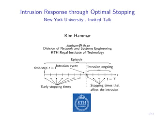
  • 1. 1/43 Intrusion Response through Optimal Stopping New York University - Invited Talk Kim Hammar kimham@kth.se Division of Network and Systems Engineering KTH Royal Institute of Technology Intrusion event time-step t = 1 Intrusion ongoing t t = T Early stopping times Stopping times that affect the intrusion Episode
  • 2. 2/43 Use Case: Intrusion Response I A Defender owns an infrastructure I Consists of connected components I Components run network services I Defender defends the infrastructure by monitoring and active defense I Has partial observability I An Attacker seeks to intrude on the infrastructure I Has a partial view of the infrastructure I Wants to compromise specific components I Attacks by reconnaissance, exploitation and pivoting Attacker Clients . . . Defender 1 IPS 1 alerts Gateway 7 8 9 10 11 6 5 4 3 2 12 13 14 15 16 17 18 19 21 23 20 22 24 25 26 27 28 29 30 31
  • 3. 3/43 Intrusion Response from the Defender’s Perspective 20 40 60 80 100 120 140 160 180 200 0.5 1 t b 20 40 60 80 100 120 140 160 180 200 50 100 150 200 t Alerts 20 40 60 80 100 120 140 160 180 200 5 10 15 t Logins
  • 4. 3/43 Intrusion Response from the Defender’s Perspective 20 40 60 80 100 120 140 160 180 200 0.5 1 t b 20 40 60 80 100 120 140 160 180 200 50 100 150 200 t Alerts 20 40 60 80 100 120 140 160 180 200 5 10 15 t Logins
  • 5. 3/43 Intrusion Response from the Defender’s Perspective 20 40 60 80 100 120 140 160 180 200 0.5 1 t b 20 40 60 80 100 120 140 160 180 200 50 100 150 200 t Alerts 20 40 60 80 100 120 140 160 180 200 5 10 15 t Logins
  • 6. 3/43 Intrusion Response from the Defender’s Perspective 20 40 60 80 100 120 140 160 180 200 0.5 1 t b 20 40 60 80 100 120 140 160 180 200 50 100 150 200 t Alerts 20 40 60 80 100 120 140 160 180 200 5 10 15 t Logins
  • 7. 3/43 Intrusion Response from the Defender’s Perspective 20 40 60 80 100 120 140 160 180 200 0.5 1 t b 20 40 60 80 100 120 140 160 180 200 50 100 150 200 t Alerts 20 40 60 80 100 120 140 160 180 200 5 10 15 t Logins
  • 8. 3/43 Intrusion Response from the Defender’s Perspective 20 40 60 80 100 120 140 160 180 200 0.5 1 t b 20 40 60 80 100 120 140 160 180 200 50 100 150 200 t Alerts 20 40 60 80 100 120 140 160 180 200 5 10 15 t Logins
  • 9. 3/43 Intrusion Response from the Defender’s Perspective 20 40 60 80 100 120 140 160 180 200 0.5 1 t b 20 40 60 80 100 120 140 160 180 200 50 100 150 200 t Alerts 20 40 60 80 100 120 140 160 180 200 5 10 15 t Logins
  • 10. 3/43 Intrusion Response from the Defender’s Perspective 20 40 60 80 100 120 140 160 180 200 0.5 1 t b 20 40 60 80 100 120 140 160 180 200 50 100 150 200 t Alerts 20 40 60 80 100 120 140 160 180 200 5 10 15 t Logins
  • 11. 3/43 Intrusion Response from the Defender’s Perspective 20 40 60 80 100 120 140 160 180 200 0.5 1 t b 20 40 60 80 100 120 140 160 180 200 50 100 150 200 t Alerts 20 40 60 80 100 120 140 160 180 200 5 10 15 t Logins When to take a defensive action? Which action to take?
  • 12. 4/43 Formulating Intrusion Response as a Stopping Problem time-step t = 1 t t = T Episode Attacker Clients . . . Defender 1 IDS 1 alerts Gateway 7 8 9 10 11 6 5 4 3 2 12 13 14 15 16 17 18 19 21 23 20 22 24 25 26 27 28 29 30 31 I The system evolves in discrete time-steps. I Defender observes the infrastructure (IDS, log files, etc.). I An intrusion occurs at an unknown time. I The defender can make L stops. I Each stop is associated with a defensive action I The final stop shuts down the infrastructure. I Based on the observations, when is it optimal to stop?
  • 13. 4/43 Formulating Intrusion Response as a Stopping Problem Intrusion event time-step t = 1 Intrusion ongoing t t = T Episode Attacker Clients . . . Defender 1 IDS 1 alerts Gateway 7 8 9 10 11 6 5 4 3 2 12 13 14 15 16 17 18 19 21 23 20 22 24 25 26 27 28 29 30 31 I The system evolves in discrete time-steps. I Defender observes the infrastructure (IDS, log files, etc.). I An intrusion occurs at an unknown time. I The defender can make L stops. I Each stop is associated with a defensive action I The final stop shuts down the infrastructure. I Based on the observations, when is it optimal to stop?
  • 14. 4/43 Formulating Intrusion Response as a Stopping Problem Intrusion event time-step t = 1 Intrusion ongoing t t = T Early stopping times Stopping times that affect the intrusion Episode Attacker Clients . . . Defender 1 IDS 1 alerts Gateway 7 8 9 10 11 6 5 4 3 2 12 13 14 15 16 17 18 19 21 23 20 22 24 25 26 27 28 29 30 31 I The system evolves in discrete time-steps. I Defender observes the infrastructure (IDS, log files, etc.). I An intrusion occurs at an unknown time. I The defender can make L stops. I Each stop is associated with a defensive action I The final stop shuts down the infrastructure. I Based on the observations, when is it optimal to stop?
  • 15. 4/43 Formulating Intrusion Response as a Stopping Problem Intrusion event time-step t = 1 Intrusion ongoing t t = T Early stopping times Stopping times that affect the intrusion Episode Attacker Clients . . . Defender 1 IDS 1 alerts Gateway 7 8 9 10 11 6 5 4 3 2 12 13 14 15 16 17 18 19 21 23 20 22 24 25 26 27 28 29 30 31 I The system evolves in discrete time-steps. I Defender observes the infrastructure (IDS, log files, etc.). I An intrusion occurs at an unknown time. I The defender can make L stops. I Each stop is associated with a defensive action I The final stop shuts down the infrastructure. I Based on the observations, when is it optimal to stop?
  • 16. 5/43 Formulating Network Intrusion as a Stopping Problem Intrusion event (1st stop) time-step t = 1 Intrusion ongoing t (2nd stop) t = T Episode Attacker Clients . . . Defender 1 IDS 1 alerts Gateway 7 8 9 10 11 6 5 4 3 2 12 13 14 15 16 17 18 19 21 23 20 22 24 25 26 27 28 29 30 31 I The system evolves in discrete time-steps. I The attacker observes the infrastructure (IDS, log files, etc.). I The first stop action decides when to intrude. I The attacker can make 2 stops. I The second stop action terminates the intrusion. I Based on the observations & the defender’s belief, when is it optimal to stop?
  • 17. 5/43 Formulating Network Intrusion as a Stopping Problem Intrusion event (1st stop) time-step t = 1 Intrusion ongoing t (2nd stop) t = T Episode Attacker Clients . . . Defender 1 IDS 1 alerts Gateway 7 8 9 10 11 6 5 4 3 2 12 13 14 15 16 17 18 19 21 23 20 22 24 25 26 27 28 29 30 31 I The system evolves in discrete time-steps. I The attacker observes the infrastructure (IDS, log files, etc.). I The first stop action decides when to intrude. I The attacker can make 2 stops. I The second stop action terminates the intrusion. I Based on the observations & the defender’s belief, when is it optimal to stop?
  • 18. 5/43 Formulating Network Intrusion as a Stopping Problem Intrusion event (1st stop) time-step t = 1 Intrusion ongoing t (2nd stop) t = T Episode Attacker Clients . . . Defender 1 IDS 1 alerts Gateway 7 8 9 10 11 6 5 4 3 2 12 13 14 15 16 17 18 19 21 23 20 22 24 25 26 27 28 29 30 31 I The system evolves in discrete time-steps. I The attacker observes the infrastructure (IDS, log files, etc.). I The first stop action decides when to intrude. I The attacker can make 2 stops. I The second stop action terminates the intrusion. I Based on the observations & the defender’s belief, when is it optimal to stop?
  • 19. 6/43 A Dynkin Game Between the Defender and the Attacker1 Attacker Defender t = 1 t = T τ1,1 τ1,2 τ1,3 τ2,1 t Stopped Game episode Intrusion I We formalize the Dynkin game as a zero-sum partially observed one-sided stochastic game. I The defender is the maximizing player I The attacker is the minimizing player 1 E.B Dynkin. “A game-theoretic version of an optimal stopping problem”. In: Dokl. Akad. Nauk SSSR 385 (1969), pp. 16–19.
  • 20. 7/43 Our Approach for Solving the Dynkin Game s1,1 s1,2 s1,3 . . . s1,n s2,1 s2,2 s2,3 . . . s2,n . . . . . . . . . . . . . . . Emulation System Target Infrastructure Model Creation & System Identification Strategy Mapping π Selective Replication Strategy Implementation π Simulation System Reinforcement Learning & Generalization Strategy evaluation & Model estimation Automation & Self-learning systems
  • 21. 7/43 Our Approach for Solving the Dynkin Game s1,1 s1,2 s1,3 . . . s1,n s2,1 s2,2 s2,3 . . . s2,n . . . . . . . . . . . . . . . Emulation System Target Infrastructure Model Creation & System Identification Strategy Mapping π Selective Replication Strategy Implementation π Simulation System Reinforcement Learning & Generalization Strategy evaluation & Model estimation Automation & Self-learning systems
  • 22. 7/43 Our Approach for Solving the Dynkin Game s1,1 s1,2 s1,3 . . . s1,n s2,1 s2,2 s2,3 . . . s2,n . . . . . . . . . . . . . . . Emulation System Target Infrastructure Model Creation & System Identification Strategy Mapping π Selective Replication Strategy Implementation π Simulation System Reinforcement Learning & Generalization Strategy evaluation & Model estimation Automation & Self-learning systems
  • 23. 7/43 Our Approach for Solving the Dynkin Game s1,1 s1,2 s1,3 . . . s1,n s2,1 s2,2 s2,3 . . . s2,n . . . . . . . . . . . . . . . Emulation System Target Infrastructure Model Creation & System Identification Strategy Mapping π Selective Replication Strategy Implementation π Simulation System Reinforcement Learning & Generalization Strategy evaluation & Model estimation Automation & Self-learning systems
  • 24. 7/43 Our Approach for Solving the Dynkin Game s1,1 s1,2 s1,3 . . . s1,n s2,1 s2,2 s2,3 . . . s2,n . . . . . . . . . . . . . . . Emulation System Target Infrastructure Model Creation & System Identification Strategy Mapping π Selective Replication Strategy Implementation π Simulation System Reinforcement Learning & Generalization Strategy evaluation & Model estimation Automation & Self-learning systems
  • 25. 7/43 Our Approach for Solving the Dynkin Game s1,1 s1,2 s1,3 . . . s1,n s2,1 s2,2 s2,3 . . . s2,n . . . . . . . . . . . . . . . Emulation System Target Infrastructure Model Creation & System Identification Strategy Mapping π Selective Replication Strategy Implementation π Simulation System Reinforcement Learning & Generalization Strategy evaluation & Model estimation Automation & Self-learning systems
  • 26. 7/43 Our Approach for Solving the Dynkin Game s1,1 s1,2 s1,3 . . . s1,n s2,1 s2,2 s2,3 . . . s2,n . . . . . . . . . . . . . . . Emulation System Target Infrastructure Model Creation & System Identification Strategy Mapping π Selective Replication Strategy Implementation π Simulation System Reinforcement Learning & Generalization Strategy evaluation & Model estimation Automation & Self-learning systems
  • 27. 7/43 Our Approach for Solving the Dynkin Game s1,1 s1,2 s1,3 . . . s1,n s2,1 s2,2 s2,3 . . . s2,n . . . . . . . . . . . . . . . Emulation System Target Infrastructure Model Creation & System Identification Strategy Mapping π Selective Replication Strategy Implementation π Simulation System Reinforcement Learning & Generalization Strategy evaluation & Model estimation Automation & Self-learning systems
  • 28. 8/43 Outline I Use Case & Approach I Use case: Intrusion response I Approach: Optimal stopping I Theoretical Background & Formal Model I Optimal stopping problem definition I Formulating the Dynkin game as a one-sided POSG I Structure of π∗ I Stopping sets Sl are connected and nested, S1 is convex. I Existence of multi-threshold best response strategies π̃1, π̃2. I Efficient Algorithms for Learning π∗ I T-SPSA: A stochastic approximation algorithm to learn π∗ I T-FP: A Fictitious-play algorithm to approximate (π∗ 1 , π∗ 2 ) I Evaluation Results I Target system, digital twin, system identification, & results I Conclusions & Future Work
  • 29. 8/43 Outline I Use Case & Approach I Use case: Intrusion response I Approach: Optimal stopping I Theoretical Background & Formal Model I Optimal stopping problem definition I Formulating the Dynkin game as a one-sided POSG I Structure of π∗ I Stopping sets Sl are connected and nested, S1 is convex. I Existence of multi-threshold best response strategies π̃1, π̃2. I Efficient Algorithms for Learning π∗ I T-SPSA: A stochastic approximation algorithm to learn π∗ I T-FP: A Fictitious-play algorithm to approximate (π∗ 1 , π∗ 2 ) I Evaluation Results I Target system, digital twin, system identification, & results I Conclusions & Future Work
  • 30. 8/43 Outline I Use Case & Approach I Use case: Intrusion response I Approach: Optimal stopping I Theoretical Background & Formal Model I Optimal stopping problem definition I Formulating the Dynkin game as a one-sided POSG I Structure of π∗ I Stopping sets Sl are connected and nested, S1 is convex. I Existence of multi-threshold best response strategies π̃1, π̃2. I Efficient Algorithms for Learning π∗ I T-SPSA: A stochastic approximation algorithm to learn π∗ I T-FP: A Fictitious-play algorithm to approximate (π∗ 1 , π∗ 2 ) I Evaluation Results I Target system, digital twin, system identification, & results I Conclusions & Future Work
  • 31. 8/43 Outline I Use Case & Approach I Use case: Intrusion response I Approach: Optimal stopping I Theoretical Background & Formal Model I Optimal stopping problem definition I Formulating the Dynkin game as a one-sided POSG I Structure of π∗ I Stopping sets Sl are connected and nested, S1 is convex. I Existence of multi-threshold best response strategies π̃1, π̃2. I Efficient Algorithms for Learning π∗ I T-SPSA: A stochastic approximation algorithm to learn π∗ I T-FP: A Fictitious-play algorithm to approximate (π∗ 1 , π∗ 2 ) I Evaluation Results I Target system, digital twin, system identification, & results I Conclusions & Future Work
  • 32. 8/43 Outline I Use Case & Approach I Use case: Intrusion response I Approach: Optimal stopping I Theoretical Background & Formal Model I Optimal stopping problem definition I Formulating the Dynkin game as a one-sided POSG I Structure of π∗ I Stopping sets Sl are connected and nested, S1 is convex. I Existence of multi-threshold best response strategies π̃1, π̃2. I Efficient Algorithms for Learning π∗ I T-SPSA: A stochastic approximation algorithm to learn π∗ I T-FP: A Fictitious-play algorithm to approximate (π∗ 1 , π∗ 2 ) I Evaluation Results I Target system, digital twin, system identification, & results I Conclusions & Future Work
  • 33. 8/43 Outline I Use Case & Approach I Use case: Intrusion response I Approach: Optimal stopping I Theoretical Background & Formal Model I Optimal stopping problem definition I Formulating the Dynkin game as a one-sided POSG I Structure of π∗ I Stopping sets Sl are connected and nested, S1 is convex. I Existence of multi-threshold best response strategies π̃1, π̃2. I Efficient Algorithms for Learning π∗ I T-SPSA: A stochastic approximation algorithm to learn π∗ I T-FP: A Fictitious-play algorithm to approximate (π∗ 1 , π∗ 2 ) I Evaluation Results I Target system, digital twin, system identification, & results I Conclusions & Future Work
  • 34. 9/43 Optimal Stopping: A Brief History I History: I Studied in the 18th century to analyze a gambler’s fortune I Formalized by Abraham Wald in 19472 I Since then it has been generalized and developed by (Chow3 , Shiryaev & Kolmogorov4 , Bather5 , Bertsekas6 , etc.) 2 Abraham Wald. Sequential Analysis. Wiley and Sons, New York, 1947. 3 Y. Chow, H. Robbins, and D. Siegmund. “Great expectations: The theory of optimal stopping”. In: 1971. 4 Albert N. Shirayev. Optimal Stopping Rules. Reprint of russian edition from 1969. Springer-Verlag Berlin, 2007. 5 John Bather. Decision Theory: An Introduction to Dynamic Programming and Sequential Decisions. USA: John Wiley and Sons, Inc., 2000. isbn: 0471976490. 6 Dimitri P. Bertsekas. Dynamic Programming and Optimal Control. 3rd. Vol. I. Belmont, MA, USA: Athena Scientific, 2005.
  • 35. 10/43 The Optimal Stopping Problem I The General Problem: I A stochastic process (st)T t=1 is observed sequentially I Two options per t: (i) continue to observe; or (ii) stop I Find the optimal stopping time τ∗ : τ∗ = arg max τ Eτ " τ−1 X t=1 γt−1 RC st st+1 + γτ−1 RS sτ sτ # (1) where RS ss0 & RC ss0 are the stop/continue rewards I The L − lth stopping time τl is: τl = inf{t : t > τl−1, at = S}, l ∈ 1, .., L, τL+1 = 0 I τl is a random variable from sample space Ω to N, which is dependent on hτ = ρ1, a1, o1, . . . , aτ−1, oτ and independent of aτ , oτ+1, . . . I We consider the class of stopping times Tt = {τ ≤ t} ∈ Fk where Fk is the natural filtration on ht. I Solution approaches: the Markovian approach and the martingale approach.
  • 36. 10/43 The Optimal Stopping Problem I The General Problem: I A stochastic process (st)T t=1 is observed sequentially I Two options per t: (i) continue to observe; or (ii) stop I Find the optimal stopping time τ∗ : τ∗ = arg max τ Eτ " τ−1 X t=1 γt−1 RC st st+1 + γτ−1 RS sτ sτ # (2) where RS ss0 & RC ss0 are the stop/continue rewards I The L − lth stopping time τl is: τl = inf{t : t > τl−1, at = S}, l ∈ 1, .., L, τL+1 = 0 I τl is a random variable from sample space Ω to N, which is dependent on hτ = ρ1, a1, o1, . . . , aτ−1, oτ and independent of aτ , oτ+1, . . . I We consider the class of stopping times Tt = {τ ≤ t} ∈ Fk where Fk is the natural filtration on ht. I Solution approaches: the Markovian approach and the martingale approach.
  • 37. 10/43 Optimal Stopping: Solution Approaches I The Markovian approach: I Model the problem as a MDP or POMDP I A policy π∗ that satisfies the Bellman-Wald equation is optimal: π∗ (s) = arg max {S,C} " E RS s | {z } stop , E RC s + γV ∗ (s0 ) | {z } continue # ∀s ∈ S I Solve by backward induction, dynamic programming, or reinforcement learning
  • 38. 10/43 Optimal Stopping: Solution Approaches I The Markovian approach: I Assume all rewards are received upon stopping: R∅ s I V ∗ (s) majorizes R∅ s if V ∗ (s) ≥ R∅ s ∀s ∈ S I V ∗ (s) is excessive if V ∗ (s) ≥ P s0 PC s0sV ∗ (s0 ) ∀s ∈ S I V ∗ (s) is the minimal excessive function which majorizes R∅ s . s R∅ s P s0 PC ss0 V ∗ (s0 ) V ∗ (s)
  • 39. 10/43 Optimal Stopping: Solution Approaches I The martingale approach: I Model the state process as an arbitrary stochastic process I The reward of the optimal stopping time is given by the smallest supermartingale that stochastically dominates the process, called the Snell envelope7 . 7 J. L. Snell. “Applications of martingale system theorems”. In: Transactions of the American Mathematical Society 73 (1952), pp. 293–312.
  • 40. 11/43 The Defender’s Optimal Stopping problem as a POMDP I States: I Intrusion state st ∈ {0, 1}, terminal ∅. I Observations: I IDS Alerts weighted by priority ot, stops remaining lt ∈ {1, .., L}, f (ot|st) I Actions: I “Stop” (S) and “Continue” (C) I Rewards: I Reward: security and service. Penalty: false alarms and intrusions I Transition probabilities: I Bernoulli process (Qt)T t=1 ∼ Ber(p) defines intrusion start It ∼ Ge(p) I Objective and Horizon: I max Eπ hPT∅ t=1 r(st, at) i , T∅ 0 1 ∅ t ≥ 1 lt 0 t ≥ 2 lt 0 intrusion starts Qt = 1 final stop lt = 0 intrusion prevented lt = 0 5 10 15 20 25 intrusion start time t 0.0 0.5 1.0 CDF I t (t) It ∼ Ge(p = 0.2)
  • 41. 11/43 The Defender’s Optimal Stopping problem as a POMDP I States: I Intrusion state st ∈ {0, 1}, terminal ∅. I Observations: I IDS Alerts weighted by priority ot, stops remaining lt ∈ {1, .., L}, f (ot|st) I Actions: I “Stop” (S) and “Continue” (C) I Rewards: I Reward: security and service. Penalty: false alarms and intrusions I Transition probabilities: I Bernoulli process (Qt)T t=1 ∼ Ber(p) defines intrusion start It ∼ Ge(p) I Objective and Horizon: I max Eπ hPT∅ t=1 r(st, at) i , T∅ 0 1 ∅ t ≥ 1 lt 0 t ≥ 2 lt 0 intrusion starts Qt = 1 final stop lt = 0 intrusion prevented lt = 0 5 10 15 20 25 intrusion start time t 0.0 0.5 1.0 CDF I t (t) It ∼ Ge(p = 0.2)
  • 42. 11/43 The Defender’s Optimal Stopping problem as a POMDP I States: I Intrusion state st ∈ {0, 1}, terminal ∅. I Observations: I IDS Alerts weighted by priority ot, stops remaining lt ∈ {1, .., L}, f (ot|st) I Actions: I “Stop” (S) and “Continue” (C) I Rewards: I Reward: security and service. Penalty: false alarms and intrusions I Transition probabilities: I Bernoulli process (Qt)T t=1 ∼ Ber(p) defines intrusion start It ∼ Ge(p) I Objective and Horizon: I max Eπ hPT∅ t=1 r(st, at) i , T∅ 0 1 ∅ t ≥ 1 lt 0 t ≥ 2 lt 0 intrusion starts Qt = 1 final stop lt = 0 intrusion prevented lt = 0 5 10 15 20 25 intrusion start time t 0.0 0.5 1.0 CDF I t (t) It ∼ Ge(p = 0.2)
  • 43. 11/43 The Defender’s Optimal Stopping problem as a POMDP I States: I Intrusion state st ∈ {0, 1}, terminal ∅. I Observations: I IDS Alerts weighted by priority ot, stops remaining lt ∈ {1, .., L}, f (ot|st) I Actions: I “Stop” (S) and “Continue” (C) I Rewards: I Reward: security and service. Penalty: false alarms and intrusions I Transition probabilities: I Bernoulli process (Qt)T t=1 ∼ Ber(p) defines intrusion start It ∼ Ge(p) I Objective and Horizon: I max Eπ hPT∅ t=1 r(st, at) i , T∅ 0 1 ∅ t ≥ 1 lt 0 t ≥ 2 lt 0 intrusion starts Qt = 1 final stop lt = 0 intrusion prevented lt = 0 5 10 15 20 25 intrusion start time t 0.0 0.5 1.0 CDF I t (t) It ∼ Ge(p = 0.2)
  • 44. 11/43 The Defender’s Optimal Stopping problem as a POMDP I States: I Intrusion state st ∈ {0, 1}, terminal ∅. I Observations: I IDS Alerts weighted by priority ot, stops remaining lt ∈ {1, .., L}, f (ot|st) I Actions: I “Stop” (S) and “Continue” (C) I Rewards: I Reward: security and service. Penalty: false alarms and intrusions I Transition probabilities: I Bernoulli process (Qt)T t=1 ∼ Ber(p) defines intrusion start It ∼ Ge(p) I Objective and Horizon: I max Eπ hPT∅ t=1 r(st, at) i , T∅ 0 1 ∅ t ≥ 1 lt 0 t ≥ 2 lt 0 intrusion starts Qt = 1 final stop lt = 0 intrusion prevented lt = 0 5 10 15 20 25 intrusion start time t 0.0 0.5 1.0 CDF I t (t) It ∼ Ge(p = 0.2)
  • 45. 11/43 The Defender’s Optimal Stopping problem as a POMDP I States: I Intrusion state st ∈ {0, 1}, terminal ∅. I Observations: I IDS Alerts weighted by priority ot, stops remaining lt ∈ {1, .., L}, f (ot|st) I Actions: I “Stop” (S) and “Continue” (C) I Rewards: I Reward: security and service. Penalty: false alarms and intrusions I Transition probabilities: I Bernoulli process (Qt)T t=1 ∼ Ber(p) defines intrusion start It ∼ Ge(p) I Objective and Horizon: I max Eπ hPT∅ t=1 r(st, at) i , T∅ 0 1 ∅ t ≥ 1 lt 0 t ≥ 2 lt 0 intrusion starts Qt = 1 final stop lt = 0 intrusion prevented lt = 0 5 10 15 20 25 intrusion start time t 0.0 0.5 1.0 CDF I t (t) It ∼ Ge(p = 0.2)
  • 46. 11/43 The Defender’s Optimal Stopping problem as a POMDP I States: I Intrusion state st ∈ {0, 1}, terminal ∅. I Observations: I IDS Alerts weighted by priority ot, stops remaining lt ∈ {1, .., L}, f (ot|st) I Actions: I “Stop” (S) and “Continue” (C) I Rewards: I Reward: security and service. Penalty: false alarms and intrusions I Transition probabilities: I Bernoulli process (Qt)T t=1 ∼ Ber(p) defines intrusion start It ∼ Ge(p) I Objective and Horizon: I max Eπ hPT∅ t=1 r(st, at) i , T∅ 0 1 ∅ t ≥ 1 lt 0 t ≥ 2 lt 0 intrusion starts Qt = 1 final stop lt = 0 intrusion prevented lt = 0 5 10 15 20 25 intrusion start time t 0.0 0.5 1.0 CDF I t (t) It ∼ Ge(p = 0.2)
  • 47. 12/43 The Attacker’s Optimal Stopping problem as an MDP I States: I Intrusion state st ∈ {0, 1}, terminal ∅, defender belief b ∈ [0, 1]. I Actions: I “Stop” (S) and “Continue” (C) I Rewards: I Reward: denial of service and intrusion. Penalty: detection I Transition probabilities: I Intrusion starts and ends when the attacker takes stop actions I Objective and Horizon: I max Eπ hPT∅ t=1 r(st, at) i , T∅ 0 1 ∅ t ≥ 1 t ≥ 2 intrusion starts at = 1 final stop detected
  • 48. 13/43 The Dynkin Game as a One-Sided POSG I Players: I Player 1 is the defender and player 2 is the attacker. Hence, N = {1, 2}. I Actions: I A1 = A2 = {S, C}. I Rewards: I Zero-sum game. Defender maximizes, attacker minimizes. I Observability: I The defender has partial observability. The attacker has full observability. I Obective functions: J1(π1, π2) = E(π1,π2) T X t=1 γt−1 R(st, at) # (3) J2(π1, π2) = −J1(π1, π2) (4) 0 1 ∅ t ≥ 1 l 0 t ≥ 2 l 0 a (2) t = S l = 1 , a ( 1 ) t = S l = 1 , a ( 1 ) t = S i n t r u s i o n s t o p p e d w . p φ l o r t e r m i n a t e d ( a ( 2 ) t = S )
  • 49. 14/43 Outline I Use Case Approach I Use case: Intrusion response I Approach: Optimal stopping I Theoretical Background Formal Model I Optimal stopping problem definition I Formulating the Dynkin game as a one-sided POSG I Structure of π∗ I Stopping sets Sl are connected and nested, S1 is convex. I Existence of multi-threshold best response strategies π̃1, π̃2. I Efficient Algorithms for Learning π∗ I T-SPSA: A stochastic approximation algorithm to learn π∗ I T-FP: A Fictitious-play algorithm to approximate (π∗ 1 , π∗ 2 ) I Evaluation Results I Target system, digital twin, system identification, results I Conclusions Future Work
  • 50. 15/43 Structural Result: Optimal Multi-Threshold Policy Theorem Given the intrusion response POMDP, the following holds: 1. Sl−1 ⊆ Sl for l = 2, . . . L. 2. If L = 1, there exists an optimal threshold α∗ ∈ [0, 1] and an optimal defender policy of the form: π∗ L(b(1)) = S ⇐⇒ b(1) ≥ α∗ (5) 3. If L ≥ 1 and fX is totally positive of order 2 (TP2), there exists L optimal thresholds α∗ l ∈ [0, 1] and an optimal defender policy of the form: π∗ l (b(1)) = S ⇐⇒ b(1) ≥ α∗ l , l = 1, . . . , L (6) where α∗ l is decreasing in l.
  • 51. 15/43 Structural Result: Optimal Multi-Threshold Policy Theorem Given the intrusion response POMDP, the following holds: 1. Sl−1 ⊆ Sl for l = 2, . . . L. 2. If L = 1, there exists an optimal threshold α∗ ∈ [0, 1] and an optimal defender policy of the form: π∗ L(b(1)) = S ⇐⇒ b(1) ≥ α∗ (7) 3. If L ≥ 1 and fX is totally positive of order 2 (TP2), there exists L optimal thresholds α∗ l ∈ [0, 1] and an optimal defender policy of the form: π∗ l (b(1)) = S ⇐⇒ b(1) ≥ α∗ l , l = 1, . . . , L (8) where α∗ l is decreasing in l.
  • 52. 15/43 Structural Result: Optimal Multi-Threshold Policy Theorem Given the intrusion response POMDP, the following holds: 1. Sl−1 ⊆ Sl for l = 2, . . . L. 2. If L = 1, there exists an optimal threshold α∗ ∈ [0, 1] and an optimal defender policy of the form: π∗ L(b(1)) = S ⇐⇒ b(1) ≥ α∗ (9) 3. If L ≥ 1 and fX is totally positive of order 2 (TP2), there exists L optimal thresholds α∗ l ∈ [0, 1] and an optimal defender policy of the form: π∗ l (b(1)) = S ⇐⇒ b(1) ≥ α∗ l , l = 1, . . . , L (10) where α∗ l is decreasing in l.
  • 53. 15/43 Structural Result: Optimal Multi-Threshold Policy Theorem Given the intrusion response POMDP, the following holds: 1. Sl−1 ⊆ Sl for l = 2, . . . L. 2. If L = 1, there exists an optimal threshold α∗ ∈ [0, 1] and an optimal defender policy of the form: π∗ L(b(1)) = S ⇐⇒ b(1) ≥ α∗ (11) 3. If L ≥ 1 and fX is totally positive of order 2 (TP2), there exists L optimal thresholds α∗ l ∈ [0, 1] and an optimal defender policy of the form: π∗ l (b(1)) = S ⇐⇒ b(1) ≥ α∗ l , l = 1, . . . , L (12) where α∗ l is decreasing in l.
  • 54. 16/43 Structural Result: Optimal Multi-Threshold Policy b(1) 0 1 belief space B = [0, 1]
  • 55. 16/43 Structural Result: Optimal Multi-Threshold Policy b(1) 0 1 belief space B = [0, 1] S1 α∗ 1
  • 56. 16/43 Structural Result: Optimal Multi-Threshold Policy b(1) 0 1 belief space B = [0, 1] S1 S2 α∗ 1 α∗ 2
  • 57. 16/43 Structural Result: Optimal Multi-Threshold Policy b(1) 0 1 belief space B = [0, 1] S1 S2 . . . SL α∗ 1 α∗ 2 α∗ L . . .
  • 58. 17/43 Lemma: V ∗ (b) is Piece-wise Linear and Convex Lemma V ∗(b) is piece-wise linear and convex. I Belief space B is the |S − 1| dimensional unit simplex. I |B| = ∞, high-dimensional (|S − 1|) continuous vector I Infinite set of deterministic policies: maxπ:B→A Eπ P t rt B(3): 2-dimensional unit-simplex 0.25 0.55 0.2 (1, 0, 0) (0, 1, 0) (0, 0, 1) (0.25, 0.55, 0.2) B(2): 1-dimensional unit-simplex (1, 0) (0, 1) 0.4 0.6 (0.4, 0.6)
  • 59. 17/43 Lemma: V ∗ (b) is Piece-wise Linear and Convex I Only finite set of belief points b ∈ B are “reachable”. I Finite horizon =⇒ finite set of “conditional plans” H → A I Set of pure strategies in an extensive game against nature N.{a1} N.{a2} N.{a3} 1.{a1, o1} 1.{a1, o2} 1.{a1, o3} 1.{a3, o3} 1.{a3, o2} 1.{a3, o1} 1.{a2, o1} 1.{a2, o2} 1.{a2, o3} 1.∅ |A| = 2, |O| = 3, T = 2 a1 a2 a3 o1 o2 o3 o1 o2 o3 o3 o2 o1 a1 a2 a1 a2 a1 a2 a1 a2 a1 a2 a1 a2 a2 a1 a2 a1 a2 a1
  • 60. 17/43 Lemma: V ∗ (b) is Piece-wise Linear and Convex I Only finite set of belief points b ∈ B are “reachable”. I Finite horizon =⇒ finite set of “conditional plans” H → A I Set of pure strategies in an extensive game against nature N.{a1} N.{a2} N.{a3} 1.{a1, o1} 1.{a1, o2} 1.{a1, o3} 1.{a3, o3} 1.{a3, o2} 1.{a3, o1} 1.{a2, o1} 1.{a2, o2} 1.{a2, o3} 1.∅ |A| = 2, |O| = 3, T = 2 Conditional plan β a1 a2 a3 o1 o2 o3 o1 o2 o3 o3 o2 o1 a1 a2 a1 a2 a1 a2 a1 a2 a1 a2 a1 a2 a2 a1 a2 a1 a2 a1
  • 61. 18/43 Lemma: V ∗ (b) is Piece-wise Linear and Convex I For each conditional plan β ∈ Γ: I Define vector αβ ∈ R|S| such that αβ i = V β (i) I =⇒ V β (b) = bT αβ (linear in b). I Thus, V ∗(b) = maxβ∈Γ bT αβ (piece-wise linear and convex8) b bα1 bα2 bα3 bα4 bα5 0
  • 62. 18/43 Lemma: V ∗ (b) is Piece-wise Linear and Convex I For each conditional plan β ∈ Γ: I Define vector αβ ∈ R|S| such that αβ i = V β (i) I =⇒ V β (b) = bT αβ (linear in b). I Thus, V ∗(b) = maxβ∈Γ bT αβ (piece-wise linear and convex9) b V ∗ (b) bα1 bα2 bα3 bα4 bα5 0
  • 63. 19/43 Proofs: S1 is convex10 I S1 is convex if: I for any two belief states b1, b2 ∈ S1 I any convex combination of b1, b2 is also in S1 I i.e. b1, b2 ∈ S1 =⇒ λb1 + (1 − λ)b2 ∈ S1 for λ ∈ [0, 1]. I Since V ∗(b) is convex: V ∗ (λb1 + (1 − λ)b2) ≤ λV ∗ (b1) + (1 − λ)V (b2) I Since b1, b2 ∈ S1: V ∗ (b1) = Q∗ (b1, S) S=stop V ∗ (b2) = Q∗ (b2, S) S=stop 10 Vikram Krishnamurthy. Partially Observed Markov Decision Processes: From Filtering to Controlled Sensing. Cambridge University Press, 2016. doi: 10.1017/CBO9781316471104.
  • 64. 19/43 Proofs: S1 is convex11 I S1 is convex if: I for any two belief states b1, b2 ∈ S1 I any convex combination of b1, b2 is also in S1 I i.e. b1, b2 ∈ S1 =⇒ λb1 + (1 − λ)b2 ∈ S1 for λ ∈ [0, 1]. I Since V ∗(b) is convex: V ∗ (λb1 + (1 − λ)b2) ≤ λV ∗ (b1) + (1 − λ)V (b2) I Since b1, b2 ∈ S1: V ∗ (b1) = Q∗ (b1, S) S=stop V ∗ (b2) = Q∗ (b2, S) S=stop 11 Vikram Krishnamurthy. Partially Observed Markov Decision Processes: From Filtering to Controlled Sensing. Cambridge University Press, 2016. doi: 10.1017/CBO9781316471104.
  • 65. 19/43 Proofs: S1 is convex12 I S1 is convex if: I for any two belief states b1, b2 ∈ S1 I any convex combination of b1, b2 is also in S1 I i.e. b1, b2 ∈ S1 =⇒ λb1 + (1 − λ)b2 ∈ S1 for λ ∈ [0, 1]. I Since V ∗(b) is convex: V ∗ (λb1 + (1 − λ)b2) ≤ λV ∗ (b1) + (1 − λ)V (b2) I Since b1, b2 ∈ S1: V ∗ (b1) = Q∗ (b1, S) S=stop V ∗ (b2) = Q∗ (b2, S) S=stop 12 Vikram Krishnamurthy. Partially Observed Markov Decision Processes: From Filtering to Controlled Sensing. Cambridge University Press, 2016. doi: 10.1017/CBO9781316471104.
  • 66. 20/43 Proofs: S1 is convex13 Proof. Assume b1, b2 ∈ S1. Then for any λ ∈ [0, 1]: V ∗ λb1(1) + (1 − λ)b2(1) ≤ λV ∗ b1(1)) + (1 − λ)V ∗ (b2(1) = λQ∗ (b1, S) + (1 − λ)Q∗ (b2, S) 13 Vikram Krishnamurthy. Partially Observed Markov Decision Processes: From Filtering to Controlled Sensing. Cambridge University Press, 2016. doi: 10.1017/CBO9781316471104.
  • 67. 20/43 Proofs: S1 is convex14 Proof. Assume b1, b2 ∈ S1. Then for any λ ∈ [0, 1]: V ∗ λb1(1) + (1 − λ)b2(1) ≤ λV ∗ b1(1)) + (1 − λ)V ∗ (b2(1) = λQ∗ (b1, S) + (1 − λ)Q∗ (b2, S) = λR∅ b1 + (1 − λ)R∅ b2 = X s (λb1(s) + (1 − λ)b2(s))R∅ s 14 Vikram Krishnamurthy. Partially Observed Markov Decision Processes: From Filtering to Controlled Sensing. Cambridge University Press, 2016. doi: 10.1017/CBO9781316471104.
  • 68. 20/43 Proofs: S1 is convex15 Proof. Assume b1, b2 ∈ S1. Then for any λ ∈ [0, 1]: V ∗ λb1(1) + (1 − λ)b2(1) ≤ λV ∗ b1(1)) + (1 − λ)V ∗ (b2(1) = λQ∗ (b1, S) + (1 − λ)Q∗ (b2, S) = λR∅ b1 + (1 − λ)R∅ b2 = X s (λb1(s) + (1 − λ)b2(s))R∅ s = Q∗ λb1 + (1 − λ)b2, S 15 Vikram Krishnamurthy. Partially Observed Markov Decision Processes: From Filtering to Controlled Sensing. Cambridge University Press, 2016. doi: 10.1017/CBO9781316471104.
  • 69. 20/43 Proofs: S1 is convex16 Proof. Assume b1, b2 ∈ S1. Then for any λ ∈ [0, 1]: V ∗ λb1(1) + (1 − λ)b2(1) ≤ λV ∗ b1(1)) + (1 − λ)V ∗ (b2(1) = λQ∗ (b1, S) + (1 − λ)Q∗ (b2, S) = λR∅ b1 + (1 − λ)R∅ b2 = X s (λb1(s) + (1 − λ)b2(s))R∅ s = Q∗ λb1 + (1 − λ)b2, S ≤ V ∗ λb1(1) + (1 − λ)b2(1) the last inequality is because V ∗ is optimal. The second-to-last is because there is just a single stop. 16 Vikram Krishnamurthy. Partially Observed Markov Decision Processes: From Filtering to Controlled Sensing. Cambridge University Press, 2016. doi: 10.1017/CBO9781316471104.
  • 70. 20/43 Proofs: S1 is convex17 Proof. Assume b1, b2 ∈ S1. Then for any λ ∈ [0, 1]: V ∗ λb1(1) + (1 − λ)b2(1) ≤ λV ∗ b1(1)) + (1 − λ)V ∗ (b2(1) = λQ∗ (b1, S) + (1 − λ)Q∗ (b2, S) = Q∗ λb1 + (1 − λ)b2, S ≤ V ∗ λb1(1) + (1 − λ)b2(1) the last inequality is because V ∗ is optimal. The second-to-last is because there is just a single stop. Hence: Q∗ λb1 + (1 − λ)b2, S = V ∗ λb1(1) + (1 − λ)b2(1) b1, b2 ∈ S1 =⇒ (λb1 + (1 − λ)) ∈ S1. Therefore S1 is convex. 17 Vikram Krishnamurthy. Partially Observed Markov Decision Processes: From Filtering to Controlled Sensing. Cambridge University Press, 2016. doi: 10.1017/CBO9781316471104.
  • 71. 20/43 Proofs: S1 is convex18 b(1) 0 1 belief space B = [0, 1] S1 α∗ 1 β∗ 1 18 Vikram Krishnamurthy. Partially Observed Markov Decision Processes: From Filtering to Controlled Sensing. Cambridge University Press, 2016. doi: 10.1017/CBO9781316471104.
  • 72. 21/43 Proofs: Single-threshold policy is optimal if L = 119 I In our case, B = [0, 1]. We know S1 is a convex subset of B. I Consequence, S1 = [α∗, β∗]. We show that β∗ = 1. I If b(1) = 1, using our definition of the reward function, the Bellman equation states: π∗ (1) ∈ arg max {S,C} 150 + V ∗ (∅) | {z } a=S , −90 + X o∈O Z(o, 1, C)V ∗ bo C (1) | {z } a=C # = arg max {S,C} 150 |{z} a=S , −90 + V ∗ (1) | {z } a=C # = S i.e π∗ (1) =Stop I Hence 1 ∈ S1. It follows that S1 = [α∗, 1] and: π∗ b(1) = ( S if b(1) ≥ α∗ C otherwise 19 Kim Hammar and Rolf Stadler. “Learning Intrusion Prevention Policies through Optimal Stopping”. In: International Conference on Network and Service Management (CNSM 2021). http://dl.ifip.org/db/conf/cnsm/cnsm2021/1570732932.pdf. Izmir, Turkey, 2021.
  • 73. 21/43 Proofs: Single-threshold policy is optimal if L = 120 I In our case, B = [0, 1]. We know S1 is a convex subset of B. I Consequence, S1 = [α∗, β∗]. We show that β∗ = 1. I If b(1) = 1, using our definition of the reward function, the Bellman equation states: π∗ (1) ∈ arg max {S,C} 150 + V ∗ (∅) | {z } a=S , −90 + X o∈O Z(o, 1, C)V ∗ bo C (1) | {z } a=C # = arg max {S,C} 150 |{z} a=S , −90 + V ∗ (1) | {z } a=C # = S i.e π∗ (1) =Stop I Hence 1 ∈ S1. It follows that S1 = [α∗, 1] and: π∗ b(1) = ( S if b(1) ≥ α∗ C otherwise 20 Kim Hammar and Rolf Stadler. “Learning Intrusion Prevention Policies through Optimal Stopping”. In: International Conference on Network and Service Management (CNSM 2021). http://dl.ifip.org/db/conf/cnsm/cnsm2021/1570732932.pdf. Izmir, Turkey, 2021.
  • 74. 21/43 Proofs: Single-threshold policy is optimal if L = 121 I In our case, B = [0, 1]. We know S1 is a convex subset of B. I Consequence, S1 = [α∗, β∗]. We show that β∗ = 1. I If b(1) = 1, using our definition of the reward function, the Bellman equation states: π∗ (1) ∈ arg max {S,C} 150 + V ∗ (∅) | {z } a=S , −90 + X o∈O Z(o, 1, C)V ∗ bo C (1) | {z } a=C # = arg max {S,C} 150 |{z} a=S , −90 + V ∗ (1) | {z } a=C # = S i.e π∗ (1) =Stop I Hence 1 ∈ S1. It follows that S1 = [α∗, 1] and: π∗ b(1) = ( S if b(1) ≥ α∗ C otherwise 21 Kim Hammar and Rolf Stadler. “Learning Intrusion Prevention Policies through Optimal Stopping”. In: International Conference on Network and Service Management (CNSM 2021). http://dl.ifip.org/db/conf/cnsm/cnsm2021/1570732932.pdf. Izmir, Turkey, 2021.
  • 75. 22/43 Proofs: Single-threshold policy is optimal if L = 1 b(1) 0 1 belief space B = [0, 1] S1 α∗ 1
  • 76. 23/43 Proofs: Nested stopping sets Sl ⊆ S1+l 22 I We want to show that Sl ⊆ S1+l I Bellman Equation: π∗ l−1(b(1)) ∈ arg max {S,C} RS b(1),l−1 + X o Po b(1)V ∗ l−2 bo (1) | {z } Stop , RC b(1),l−1 + X o Po b(1)V ∗ l−1 bo (1) | {z } Continue # I =⇒ optimal to stop if: RS b(1),l−1 − RC b(1),l−1 ≥ X o Po b(1) V ∗ l−1 bo (1) − V ∗ l−2 bo (1) 13 I Hence, if b(1) ∈ Sl−1, then (13) holds. 22 T. Nakai. “The problem of optimal stopping in a partially observable Markov chain”. In: Journal of Optimization Theory and Applications 45.3 (1985), pp. 425–442. issn: 1573-2878. doi: 10.1007/BF00938445. url: https://doi.org/10.1007/BF00938445.
  • 77. 23/43 Proofs: Nested stopping sets Sl ⊆ S1+l 23 I We want to show that Sl ⊆ S1+l I Bellman Equation: π∗ l−1(b(1)) ∈ arg max {S,C} RS b(1),l−1 + X o Po b(1)V ∗ l−2 bo (1) | {z } Stop , RC b(1),l−1 + X o Po b(1)V ∗ l−1 bo (1) | {z } Continue # I =⇒ optimal to stop if: RS b(1),l−1 − RC b(1),l−1 ≥ X o Po b(1) V ∗ l−1 bo (1) − V ∗ l−2 bo (1) 13 I Hence, if b(1) ∈ Sl−1, then (13) holds. 23 T. Nakai. “The problem of optimal stopping in a partially observable Markov chain”. In: Journal of Optimization Theory and Applications 45.3 (1985), pp. 425–442. issn: 1573-2878. doi: 10.1007/BF00938445. url: https://doi.org/10.1007/BF00938445.
  • 78. 23/43 Proofs: Nested stopping sets Sl ⊆ S1+l 24 I We want to show that Sl ⊆ S1+l I Bellman Equation: π∗ l−1(b(1)) ∈ arg max {S,C} RS b(1),l−1 + X o Po b(1)V ∗ l−2 bo (1) | {z } Stop , RC b(1),l−1 + X o Po b(1)V ∗ l−1 bo (1) | {z } Continue # I =⇒ optimal to stop if: RS b(1),l−1 − RC b(1),l−1 ≥ X o Po b(1) V ∗ l−1 bo (1) − V ∗ l−2 bo (1) (13) I Hence, if b(1) ∈ Sl−1, then (13) holds. 24 T. Nakai. “The problem of optimal stopping in a partially observable Markov chain”. In: Journal of Optimization Theory and Applications 45.3 (1985), pp. 425–442. issn: 1573-2878. doi: 10.1007/BF00938445. url: https://doi.org/10.1007/BF00938445.
  • 79. 23/43 Proofs: Nested stopping sets Sl ⊆ S1+l 25 I RS b(1) − RC b(1) ≥ X o Po b(1) V ∗ l−1 bo (1) − V ∗ l−2 bo (1) I We want to show that b(1) ∈ Sl−2 =⇒ b(1) ∈ Sl−1. I Sufficient to show that LHS above is non-decreasing in l and RHS is non-increasing in l. I LHS is non-decreasing by definition of reward function. I We show that RHS is non-increasing by induction on k = 0, 1 . . . where k is the iteration of value iteration. I We know limk→∞ V k(b) = V ∗(b). I Define W k l b(1) = V k l b(1) − V k l−1 b(1) 25 T. Nakai. “The problem of optimal stopping in a partially observable Markov chain”. In: Journal of Optimization Theory and Applications 45.3 (1985), pp. 425–442. issn: 1573-2878. doi: 10.1007/BF00938445. url: https://doi.org/10.1007/BF00938445.
  • 80. 23/43 Proofs: Nested stopping sets Sl ⊆ S1+l 26 I RS b(1) − RC b(1) ≥ X o Po b(1) V ∗ l−1 bo (1) − V ∗ l−2 bo (1) I We want to show that b(1) ∈ Sl−2 =⇒ b(1) ∈ Sl−1. I Sufficient to show that LHS above is non-decreasing in l and RHS is non-increasing in l. I LHS is non-decreasing by definition of reward function. I We show that RHS is non-increasing by induction on k = 0, 1 . . . where k is the iteration of value iteration. I We know limk→∞ V k(b) = V ∗(b). I Define W k l b(1) = V k l b(1) − V k l−1 b(1) 26 T. Nakai. “The problem of optimal stopping in a partially observable Markov chain”. In: Journal of Optimization Theory and Applications 45.3 (1985), pp. 425–442. issn: 1573-2878. doi: 10.1007/BF00938445. url: https://doi.org/10.1007/BF00938445.
  • 81. 23/43 Proofs: Nested stopping sets Sl ⊆ S1+l 27 I RS b(1) − RC b(1) ≥ X o Po b(1) V ∗ l−1 bo (1) − V ∗ l−2 bo (1) I We want to show that b(1) ∈ Sl−2 =⇒ b(1) ∈ Sl−1. I Sufficient to show that LHS above is non-decreasing in l and RHS is non-increasing in l. I LHS is non-decreasing by definition of reward function. I We show that RHS is non-increasing by induction on k = 0, 1 . . . where k is the iteration of value iteration. I We know limk→∞ V k(b) = V ∗(b). I Define W k l b(1) = V k l b(1) − V k l−1 b(1) 27 T. Nakai. “The problem of optimal stopping in a partially observable Markov chain”. In: Journal of Optimization Theory and Applications 45.3 (1985), pp. 425–442. issn: 1573-2878. doi: 10.1007/BF00938445. url: https://doi.org/10.1007/BF00938445.
  • 82. 23/43 Proofs: Nested stopping sets Sl ⊆ S1+l 28 Proof. W 0 l b(1) = 0 ∀l. Assume W k−1 l−1 b(1) − W k−1 l b(1) ≥ 0. 28 T. Nakai. “The problem of optimal stopping in a partially observable Markov chain”. In: Journal of Optimization Theory and Applications 45.3 (1985), pp. 425–442. issn: 1573-2878. doi: 10.1007/BF00938445. url: https://doi.org/10.1007/BF00938445.
  • 83. 23/43 Proofs: Nested stopping sets Sl ⊆ S1+l 29 Proof. W 0 l b(1) = 0 ∀l. Assume W k−1 l−1 b(1) − W k−1 l b(1) ≥ 0. W k l−1 b(1) − W k l (b(1)) = 2V k l−1 − V k l−2 − V k l 29 T. Nakai. “The problem of optimal stopping in a partially observable Markov chain”. In: Journal of Optimization Theory and Applications 45.3 (1985), pp. 425–442. issn: 1573-2878. doi: 10.1007/BF00938445. url: https://doi.org/10.1007/BF00938445.
  • 84. 23/43 Proofs: Nested stopping sets Sl ⊆ S1+l 30 Proof. W 0 l b(1) = 0 ∀l. Assume W k−1 l−1 b(1) − W k−1 l b(1) ≥ 0. W k l−1 b(1) − W k l (b(1)) = 2V k l−1 − V k l−2 − V k l = 2R ak l−1 b(1) − R ak l b(1) − R ak l−2 b(1) + X o∈O Po b(1) 2V k−1 l−1−ak l−1 b(1) − V k−1 l−ak l b(1) − V k−1 l−2−ak l−2 b(1) Want to show that the above is non-negative. This depends on ak l , ak l−1, ak l−2. 30 T. Nakai. “The problem of optimal stopping in a partially observable Markov chain”. In: Journal of Optimization Theory and Applications 45.3 (1985), pp. 425–442. issn: 1573-2878. doi: 10.1007/BF00938445. url: https://doi.org/10.1007/BF00938445.
  • 85. 23/43 Proofs: Nested stopping sets Sl ⊆ S1+l 31 Proof. W 0 l b(1) = 0 ∀l. Assume W k−1 l−1 b(1) − W k−1 l b(1) ≥ 0. W k l−1 b(1) − W k l (b(1)) = 2V k l−1 − V k l−2 − V k l = 2R ak l−1 b(1) − R ak l b(1) − R ak l−2 b(1) + X o∈O Po b(1) 2V k−1 l−1−ak l−1 b(1) − V k−1 l−ak l b(1) − V k−1 l−2−ak l−2 b(1) Want to show that the above is non-negative. This depends on ak l , ak l−1, ak l−2. There are four cases to consider: (1) b(1) ∈ S k l ∩ S k l−1 ∩ S k l−2; (2) b(1) ∈ S k l ∩ C k l−1 ∩ C k l−2; (3) b(1) ∈ S k l ∩ S k l−1 ∩ C k l−2; (4) b(1) ∈ C k l ∩ C k l−1 ∩ C k l−2. The other cases, e.g. b(1) ∈ S k l ∩ C k l−1 ∩ S k l−2, can be discarded due to the induction assumption.
  • 86. 23/43 Proofs: Nested stopping sets Sl ⊆ S1+l 32 Proof. If b(1) ∈ S k l ∩ S k l−1 ∩ S k l−2, then: W k l−1 b(1) − W k l b(1) = X o∈O Po b(1) W k−1 l−2 bo (1) − W k−1 l−1 bo (1) which is non-negative by the induction hypothesis. 32 T. Nakai. “The problem of optimal stopping in a partially observable Markov chain”. In: Journal of Optimization Theory and Applications 45.3 (1985), pp. 425–442. issn: 1573-2878. doi: 10.1007/BF00938445. url: https://doi.org/10.1007/BF00938445.
  • 87. 23/43 Proofs: Nested stopping sets Sl ⊆ S1+l 33 Proof. If b(1) ∈ S k l ∩ S k l−1 ∩ S k l−2, then: W k l−1 b(1) − W k l b(1) = X o∈O Po b(1) W k−1 l−2 bo (1) − W k−1 l−1 bo (1) which is non-negative by the induction hypothesis. If b(1) ∈ S k l ∩ C k l−1 ∩ C k l−2, then: W k l b(1) − W k l−1 b(1) = RC b(1) − RS b(1) + X o∈O Po b(1) W k−1 l−1 bo (1) 33 T. Nakai. “The problem of optimal stopping in a partially observable Markov chain”. In: Journal of Optimization Theory and Applications 45.3 (1985), pp. 425–442. issn: 1573-2878. doi: 10.1007/BF00938445. url: https://doi.org/10.1007/BF00938445.
  • 88. 23/43 Proofs: Nested stopping sets Sl ⊆ S1+l 34 Proof. If b(1) ∈ S k l ∩ S k l−1 ∩ S k l−2, then: W k l−1 b(1) − W k l b(1) = X o∈O Po b(1) W k−1 l−2 bo (1) − W k−1 l−1 bo (1) which is non-negative by the induction hypothesis. If b(1) ∈ S k l ∩ C k l−1 ∩ C k l−2, then: W k l b(1) − W k l−1 b(1) = RC b(1) − RS b(1) + X o∈O Po b(1) W k−1 l−1 bo (1) Bellman eq. implies, if b(1) ∈ Cl−1, then: RC b(1) − RS b(1) + X o∈O Po b(1) W k−1 l−1 bo (1) ≥ 0
  • 89. 23/43 Proofs: Nested stopping sets Sl ⊆ S1+l 35 Proof. If b(1) ∈ S k l ∩ S k l−1 ∩ C k l−2, then: W k l−1 b(1) − W k l b(1) = RS b(1) − RC b(1) − X o∈O Po b(1) W k−1 l−1 bo (1) 35 T. Nakai. “The problem of optimal stopping in a partially observable Markov chain”. In: Journal of Optimization Theory and Applications 45.3 (1985), pp. 425–442. issn: 1573-2878. doi: 10.1007/BF00938445. url: https://doi.org/10.1007/BF00938445.
  • 90. 23/43 Proofs: Nested stopping sets Sl ⊆ S1+l 36 Proof. If b(1) ∈ S k l ∩ S k l−1 ∩ C k l−2, then: W k l−1 b(1) − W k l b(1) = RS b(1) − RC b(1) − X o∈O Po b(1) W k−1 l−1 bo (1) Bellman eq. implies, if b(1) ∈ S k l−1, then: RS b(1) − RC b(1) − X o∈O Po b(1) W k−1 l−1 bo (1) ≥ 0 36 T. Nakai. “The problem of optimal stopping in a partially observable Markov chain”. In: Journal of Optimization Theory and Applications 45.3 (1985), pp. 425–442. issn: 1573-2878. doi: 10.1007/BF00938445. url: https://doi.org/10.1007/BF00938445.
  • 91. 23/43 Proofs: Nested stopping sets Sl ⊆ S1+l 37 Proof. If b(1) ∈ S k l ∩ S k l−1 ∩ C k l−2, then: W k l−1 b(1) − W k l b(1) = RS b(1) − RC b(1) − X o∈O Po b(1) W k−1 l−1 bo (1) Bellman eq. implies, if b(1) ∈ S k l−1, then: RS b(1) − RC b(1) − X o∈O Po b(1) W k−1 l−1 bo (1) ≥ 0 If b(1) ∈ C k l ∩ C k l−1 ∩ C k l−2, then: W k l−1 b(1) − W k l b(1) = X o∈O Po b(1) W k−1 l−1 bo (1) − W k−1 l bo (1) which is non-negative by the induction hypothesis. 37 T. Nakai. “The problem of optimal stopping in a partially observable Markov chain”. In: Journal of Optimization Theory and Applications 45.3 (1985), pp. 425–442. issn: 1573-2878. doi: 10.1007/BF00938445.
  • 92. 24/43 Proofs: Nested stopping sets Sl ⊆ S1+l 38 S1 ⊆ S2 still allows: b(1) 0 1 S1 S2 S2 We need to show that Sl is connected, for all l ∈ {1, . . . , L}. 38 T. Nakai. “The problem of optimal stopping in a partially observable Markov chain”. In: Journal of Optimization Theory and Applications 45.3 (1985), pp. 425–442. issn: 1573-2878. doi: 10.1007/BF00938445. url: https://doi.org/10.1007/BF00938445.
  • 93. 25/43 Proofs: Connected stopping sets Sl 39 I Sl is connected if b(1) ∈ Sl , b0(1) ≥ b(1) =⇒ b0(1) ∈ Sl I If b(1) ∈ Sl we use the Bellman eq. to obtain: RS b(1) − RC b(1) + X o Po b(1) V ∗ l−1 bo (1) − V ∗ l bo (1) ≥ 0 I We need to show that the above inequality holds for any b0(1) ≥ b(1) 39 Kim Hammar and Rolf Stadler. “Intrusion Prevention Through Optimal Stopping”. In: IEEE Transactions on Network and Service Management 19.3 (2022), pp. 2333–2348. doi: 10.1109/TNSM.2022.3176781.
  • 94. 26/43 Proofs: Monotone belief update Lemma (Monotone belief update) Given two beliefs b1(1) ≥ b2(1), if the transition probabilities and the observation probabilities are Totally Positive of Order 2 (TP2), then bo a,1(1) ≥ bo a,2(1), where bo a,1(1) and bo a,2(1) denote the beliefs updated with the Bayesian filter after taking action a ∈ A and observing o ∈ O. See Theorem 10.3.1 and proof on pp 225,238 in40 40 Vikram Krishnamurthy. Partially Observed Markov Decision Processes: From Filtering to Controlled Sensing. Cambridge University Press, 2016. doi: 10.1017/CBO9781316471104.
  • 95. 27/43 Proofs: Necessary Condition, Total Positivity of Order 241 I A row-stochastic matrix is totally positive of order 2 (TP2) if: I The rows of the matrix are stochastically monotone I Equivalently, all second-order minors are non-negative. I Example: A =    0.3 0.5 0.2 0.2 0.4 0.4 0.1 0.2 0.7    (14) There are 3 2 2 second-order minors: det 0.3 0.5 0.2 0.4 # = 0.02, det 0.2 0.4 0.1 0.2 # = 0, ...etc. (15) Since all minors are non-negative, the matrix is TP2 41 Samuel Karlin. “Total positivity, absorption probabilities and applications”. In: Transactions of the American Mathematical Society 111 (1964).
  • 96. 28/43 Proofs: Connected stopping sets Sl 42 I Since the transition probabilities are TP2 by definition and we assume the observation probabilities are TP2, the condition for showing that the stopping sets are connected reduces to the following. I Show that the below expression is weakly increasing in b(1). RS b(1) − RC b(1) + V ∗ l−1 b(1) − V ∗ l b(1) I We prove this by induction on k. 42 Kim Hammar and Rolf Stadler. “Intrusion Prevention Through Optimal Stopping”. In: IEEE Transactions on Network and Service Management 19.3 (2022), pp. 2333–2348. doi: 10.1109/TNSM.2022.3176781.
  • 97. 29/43 Proofs: Connected stopping sets Sl 43 Assume RS b(1) − RC b(1) + V k−1 l−1 b(1) − V k−1 l b(1) is weakly increasing in b(1). RS b(1) − RC b(1) + V k l−1 b(1) − V k l b(1) = RS b(1) − RC b(1)+ R ak l−1 b(1) − R ak l b(1) + X o∈O Po b(1) V k−1 l−1−ak l−1 bo (1) − V k−1 l−ak l bo (1) 43 Kim Hammar and Rolf Stadler. “Intrusion Prevention Through Optimal Stopping”. In: IEEE Transactions on Network and Service Management 19.3 (2022), pp. 2333–2348. doi: 10.1109/TNSM.2022.3176781.
  • 98. 29/43 Proofs: Connected stopping sets Sl 44 Assume RS b(1) − RC b(1) + V k−1 l−1 b(1) − V k−1 l b(1) is weakly increasing in b(1). RS b(1) − RC b(1) + V k l−1 b(1) − V k l b(1) = RS b(1) − RC b(1)+ R ak l−1 b(1) − R ak l b(1) + X o∈O Po b(1) V k−1 l−1−ak l−1 bo (1) − V k−1 l−ak l bo (1) Want to show that the above is weakly-increasing in b(1). This depends on ak l and ak l−1. 44 Kim Hammar and Rolf Stadler. “Intrusion Prevention Through Optimal Stopping”. In: IEEE Transactions on Network and Service Management 19.3 (2022), pp. 2333–2348. doi: 10.1109/TNSM.2022.3176781.
  • 99. 29/43 Proofs: Connected stopping sets Sl 45 Assume RS b(1) − RC b(1) + V k−1 l−1 b(1) − V k−1 l b(1) is weakly increasing in b(1). RS b(1) − RC b(1) + V k l−1 b(1) − V k l b(1) = RS b(1) − RC b(1)+ R ak l−1 b(1) − R ak l b(1) + X o∈O Po b(1) V k−1 l−1−ak l−1 bo (1) − V k−1 l−ak l bo (1) Want to show that the above is weakly-increasing in b(1). This depends on ak l and ak l−1. There are three cases to consider: 1. b(1) ∈ S k l ∩ S k l−1 2. b(1) ∈ S k l ∩ C k l−1 3. b(1) ∈ C k l ∩ C k l−1 45 Kim Hammar and Rolf Stadler. “Intrusion Prevention Through Optimal Stopping”. In: IEEE Transactions on Network and Service Management 19.3 (2022), pp. 2333–2348. doi: 10.1109/TNSM.2022.3176781.
  • 100. 30/43 Proofs: Connected stopping sets Sl 46 Proof. If b(1) ∈ Sl ∩ Sl−1, then: RS b(1) − RC b(1) + V k l−1 b(1) − V k l b(1) = RS b(1) − RC b(1) X o∈O Po b(1) V k−1 l−2 bo (1) − V k−1 l−1 bo (1) which is weakly increasing in b(1) by the induction hypothesis. 46 Kim Hammar and Rolf Stadler. “Intrusion Prevention Through Optimal Stopping”. In: IEEE Transactions on Network and Service Management 19.3 (2022), pp. 2333–2348. doi: 10.1109/TNSM.2022.3176781.
  • 101. 30/43 Proofs: Connected stopping sets Sl 47 Proof. If b(1) ∈ S k l ∩ S k l−1, then: RS b(1) − RC b(1) + V k l−1 b(1) − V k l b(1) = RS b(1) − RC b(1) X o∈O Po b(1) V k−1 l−2 bo (1) − V k−1 l−1 bo (1) which is weakly increasing in b(1) by the induction hypothesis. If b(1) ∈ S k l ∩ C k l−1, then: RS b(1) − RC b(1) + V k l−1 b(1) − V k l b(1) = X o∈O Po b(1) V k−1 l−1 bo (1) − V k−1 l−1 bo (1) = 0 which is trivially weakly increasing in b(1). 47 Kim Hammar and Rolf Stadler. “Intrusion Prevention Through Optimal Stopping”. In: IEEE Transactions on Network and Service Management 19.3 (2022), pp. 2333–2348. doi: 10.1109/TNSM.2022.3176781.
  • 102. 30/43 Proofs: Connected stopping sets Sl 48 Proof. If b(1) ∈ C k l ∩ C k l−1, then: RS b(1) − RC b(1) + V k l−1 b(1) − V k l b(1) = RS b(1) − RC b(1) X o∈O Po b(1) V k−1 l−1 bo (1) − V k−1 l bo (1) which is weakly increasing in b(1) by the induction hypothesis. Hence, if b(1) ∈ Sl and b0(1) ≥ b(1) then b0(1) ∈ Sl . Therefore, Sl is connected. 48 Kim Hammar and Rolf Stadler. “Intrusion Prevention Through Optimal Stopping”. In: IEEE Transactions on Network and Service Management 19.3 (2022), pp. 2333–2348. doi: 10.1109/TNSM.2022.3176781.
  • 103. 31/43 Proofs: Optimal multi-threshold policy π∗ l 49 We have shown that: I S1 = [α∗ 1, 1] I Sl ⊆ Sl+1 I Sl is connected (convex) for l = 1, . . . , L It follows that, Sl = [α∗ l , 1] and α∗ 1 ≥ α∗ 2 ≥ . . . ≥ α∗ L. b(1) 0 1 belief space B = [0, 1] S1 S2 . . . SL α∗ 1 α∗ 2 α∗ L . . . 49 Kim Hammar and Rolf Stadler. “Intrusion Prevention Through Optimal Stopping”. In: IEEE Transactions on Network and Service Management 19.3 (2022), pp. 2333–2348. doi: 10.1109/TNSM.2022.3176781.
  • 104. 32/43 Structural Result: Best Response Multi-Threshold Attacker Strategy Theorem Given the intrusion MDP, the following holds: 1. Given a defender strategy π1 ∈ Π1 where π1(S|b(1)) is non-decreasing in b(1) and π1(S|1) = 1, then there exist values β̃0,1, β̃1,1, . . ., β̃0,L, β̃1,L ∈ [0, 1] and a best response strategy π̃2 ∈ B2(π1) for the attacker that satisfies π̃2,l (0, b(1)) = C ⇐⇒ π1,l (S|b(1)) ≥ β̃0,l (16) π̃2,l (1, b(1)) = S ⇐⇒ π1,l (S|b(1)) ≥ β̃1,l (17) for l ∈ {1, . . . , L}. Proof. Follows the same idea as the proof for the defender case. See50. 50 Kim Hammar and Rolf Stadler. Learning Near-Optimal Intrusion Responses Against Dynamic Attackers. 2023.
  • 105. 33/43 Outline I Use Case Approach I Use case: Intrusion response I Approach: Optimal stopping I Theoretical Background Formal Model I Optimal stopping problem definition I Formulating the Dynkin game as a one-sided POSG I Structure of π∗ I Stopping sets Sl are connected and nested, S1 is convex. I Existence of multi-threshold best response strategies π̃1, π̃2. I Efficient Algorithms for Learning π∗ I T-SPSA: A stochastic approximation algorithm to learn π∗ I T-FP: A Fictitious-play algorithm to approximate (π∗ 1 , π∗ 2 ) I Evaluation Results I Target system, digital twin, system identification, results I Conclusions Future Work
  • 106. 34/43 Threshold-SPSA to Learn Best Responses 0.5 1 0.5 1 π̃1,l,θ̃(1) (S|b(1)) threshold σ(θ̃ (1) l ) b(1) 0 A mixed threshold strategy where σ(θ̃ (1) l ) is the threshold. I Parameterizes π̃i through threshold vectors according to Theorem 1: ϕ(a, b) , 1 + b(1 − σ(a)) σ(a)(1 − b) −20 !−1 (18) π̃i,θ̃(i) S|b(1) , ϕ θ̃ (i) l , b(1) (19) I The parameterized strategies are mixed (and differentiable) strategies that approximate threshold strategies. I Update threshold vectors θ(i) using SPSA iteratively.
  • 107. 35/43 Threshold-Fictitious Play to Approximate an Equilibrium π̃2 ∈ B2(π1) π2 π1 π̃1 ∈ B1(π2) π̃0 2 ∈ B2(π0 1) π0 2 π0 1 π̃0 1 ∈ B1(π0 2) . . . π∗ 2 ∈ B2(π∗ 1) π∗ 1 ∈ B1(π∗ 2) Fictitious play: iterative averaging of best responses. I Learn best response strategies iteratively through T-SPSA I Average best responses to approximate the equilibrium
  • 108. 36/43 Comparison against State-of-the-art Algorithms 0 10 20 30 40 50 60 training time (min) 0 50 100 Reward per episode against Novice 0 10 20 30 40 50 60 training time (min) Reward per episode against Experienced 0 10 20 30 40 50 60 training time (min) Reward per episode against Expert PPO ThresholdSPSA Shiryaev’s Algorithm (α = 0.75) HSVI upper bound
  • 109. 37/43 Outline I Use Case Approach I Use case: Intrusion response I Approach: Optimal stopping I Theoretical Background Formal Model I Optimal stopping problem definition I Formulating the Dynkin game as a one-sided POSG I Structure of π∗ I Stopping sets Sl are connected and nested, S1 is convex. I Existence of multi-threshold best response strategies π̃1, π̃2. I Efficient Algorithms for Learning π∗ I T-SPSA: A stochastic approximation algorithm to learn π∗ I T-FP: A Fictitious-play algorithm to approximate (π∗ 1 , π∗ 2 ) I Evaluation Results I Target system, digital twin, system identification, results I Conclusions Future Work
  • 110. 37/43 Outline I Use Case Approach I Use case: Intrusion response I Approach: Optimal stopping I Theoretical Background Formal Model I Optimal stopping problem definition I Formulating the Dynkin game as a one-sided POSG I Structure of π∗ I Stopping sets Sl are connected and nested, S1 is convex. I Existence of multi-threshold best response strategies π̃1, π̃2. I Efficient Algorithms for Learning π∗ I T-SPSA: A stochastic approximation algorithm to learn π∗ I T-FP: A Fictitious-play algorithm to approximate (π∗ 1 , π∗ 2 ) I Evaluation Results I Target system, digital twin, system identification, results I Conclusions Future Work
  • 111. 38/43 Creating a Digital Twin of the Target Infrastructure s1,1 s1,2 s1,3 . . . s1,n s2,1 s2,2 s2,3 . . . s2,n . . . . . . . . . . . . . . . Emulation System Target Infrastructure Model Creation System Identification Strategy Mapping π Selective Replication Strategy Implementation π Simulation System Reinforcement Learning Generalization Strategy evaluation Model estimation Automation Self-learning systems
  • 112. 39/43 Creating a Digital Twin of the Target Infrastructure I Emulate hosts with docker containers I Emulate IPS and vulnerabilities with software I Network isolation and traffic shaping through NetEm in the Linux kernel I Enforce resource constraints using cgroups. I Emulate client arrivals with Poisson process I Internal connections are full-duplex loss-less with bit capacities of 1000 Mbit/s I External connections are full-duplex with bit capacities of 100 Mbit/s 0.1% packet loss in normal operation and random bursts of 1% packet loss Attacker Clients . . . Defender 1 IPS 1 alerts Gateway 7 8 9 10 11 6 5 4 3 2 12 13 14 15 16 17 18 19 21 23 20 22 24 25 26 27 28 29 30 31
  • 113. 39/43 Creating a Digital Twin of the Target Infrastructure I Emulate hosts with docker containers I Emulate IPS and vulnerabilities with software I Network isolation and traffic shaping through NetEm in the Linux kernel I Enforce resource constraints using cgroups. I Emulate client arrivals with Poisson process I Internal connections are full-duplex loss-less with bit capacities of 1000 Mbit/s I External connections are full-duplex with bit capacities of 100 Mbit/s 0.1% packet loss in normal operation and random bursts of 1% packet loss Attacker Clients . . . Defender 1 IPS 1 alerts Gateway 7 8 9 10 11 6 5 4 3 2 12 13 14 15 16 17 18 19 21 23 20 22 24 25 26 27 28 29 30 31
  • 114. 39/43 Creating a Digital Twin of the Target Infrastructure I Emulate hosts with docker containers I Emulate IPS and vulnerabilities with software I Network isolation and traffic shaping through NetEm in the Linux kernel I Enforce resource constraints using cgroups. I Emulate client arrivals with Poisson process I Internal connections are full-duplex loss-less with bit capacities of 1000 Mbit/s I External connections are full-duplex with bit capacities of 100 Mbit/s 0.1% packet loss in normal operation and random bursts of 1% packet loss Attacker Clients . . . Defender 1 IPS 1 alerts Gateway 7 8 9 10 11 6 5 4 3 2 12 13 14 15 16 17 18 19 21 23 20 22 24 25 26 27 28 29 30 31
  • 115. 39/43 Creating a Digital Twin of the Target Infrastructure I Emulate hosts with docker containers I Emulate IPS and vulnerabilities with software I Network isolation and traffic shaping through NetEm in the Linux kernel I Enforce resource constraints using cgroups. I Emulate client arrivals with Poisson process I Internal connections are full-duplex loss-less with bit capacities of 1000 Mbit/s I External connections are full-duplex with bit capacities of 100 Mbit/s 0.1% packet loss in normal operation and random bursts of 1% packet loss Attacker Clients . . . Defender 1 IPS 1 alerts Gateway 7 8 9 10 11 6 5 4 3 2 12 13 14 15 16 17 18 19 21 23 20 22 24 25 26 27 28 29 30 31
  • 116. 39/43 Creating a Digital Twin of the Target Infrastructure I Emulate hosts with docker containers I Emulate IPS and vulnerabilities with software I Network isolation and traffic shaping through NetEm in the Linux kernel I Enforce resource constraints using cgroups. I Emulate client arrivals with Poisson process I Internal connections are full-duplex loss-less with bit capacities of 1000 Mbit/s I External connections are full-duplex with bit capacities of 100 Mbit/s 0.1% packet loss in normal operation and random bursts of 1% packet loss Attacker Clients . . . Defender 1 IPS 1 alerts Gateway 7 8 9 10 11 6 5 4 3 2 12 13 14 15 16 17 18 19 21 23 20 22 24 25 26 27 28 29 30 31
  • 117. 39/43 Creating a Digital Twin of the Target Infrastructure I Emulate hosts with docker containers I Emulate IPS and vulnerabilities with software I Network isolation and traffic shaping through NetEm in the Linux kernel I Enforce resource constraints using cgroups. I Emulate client arrivals with Poisson process I Internal connections are full-duplex loss-less with bit capacities of 1000 Mbit/s I External connections are full-duplex with bit capacities of 100 Mbit/s 0.1% packet loss in normal operation and random bursts of 1% packet loss Attacker Clients . . . Defender 1 IPS 1 alerts Gateway 7 8 9 10 11 6 5 4 3 2 12 13 14 15 16 17 18 19 21 23 20 22 24 25 26 27 28 29 30 31
  • 118. 39/43 Our Approach for Automated Network Security s1,1 s1,2 s1,3 . . . s1,n s2,1 s2,2 s2,3 . . . s2,n . . . . . . . . . . . . . . . Emulation System Target Infrastructure Model Creation System Identification Strategy Mapping π Selective Replication Strategy Implementation π Simulation System Reinforcement Learning Generalization Strategy evaluation Model estimation Automation Self-learning systems
  • 119. 40/43 System Identification ˆ f O (o t |0) Probability distribution of # IPS alerts weighted by priority ot 0 1000 2000 3000 4000 5000 6000 7000 8000 9000 ˆ f O (o t |1) Fitted model Distribution st = 0 Distribution st = 1 I The distribution fO of defender observations (system metrics) is unknown. I We fit a Gaussian mixture distribution ˆ fO as an estimate of fO in the target infrastructure. I For each state s, we obtain the conditional distribution ˆ fO|s through expectation-maximization.
  • 120. 41/43 Learning Curves in Simulation and Digital Twin 0 50 100 Novice Reward per episode 0 50 100 Episode length (steps) 0.0 0.5 1.0 P[intrusion interrupted] 0.0 0.5 1.0 1.5 P[early stopping] 5 10 Duration of intrusion −50 0 50 100 experienced 0 50 100 150 0.0 0.5 1.0 0.0 0.5 1.0 1.5 0 5 10 0 20 40 60 training time (min) −50 0 50 100 expert 0 20 40 60 training time (min) 0 50 100 150 0 20 40 60 training time (min) 0.0 0.5 1.0 0 20 40 60 training time (min) 0.0 0.5 1.0 1.5 2.0 0 20 40 60 training time (min) 0 5 10 15 20 πθ,l simulation πθ,l emulation (∆x + ∆y) ≥ 1 baseline Snort IPS upper bound
  • 121. 42/43 Conclusions I We develop a method to automatically learn security strategies. I We apply the method to an intrusion response use case. I We design a solution framework guided by the theory of optimal stopping. I We present several theoretical results on the structure of the optimal solution. I We show numerical results in a realistic emulation environment. s1,1 s1,2 s1,3 . . . s1,n s2,1 s2,2 s2,3 . . . s2,n . . . . . . . . . . . . . . . Emulation Target System Model Creation System Identification Strategy Mapping π Selective Replication Strategy Implementation π Simulation Learning
  • 122. 43/43 Current and Future Work Time st st+1 st+2 st+3 . . . rt+1 rt+2 rt+3 rrT 1. Extend use case I Additional defender actions I Utilize SDN controller and NFV-based defenses I Increase observation space and attacker model I More heterogeneous client population 2. Extend solution framework I Model-predictive control I Rollout-based techniques I Extend system identification algorithm 3. Extend theoretical results I Exploit symmetries and causal structure I Utilize theory to improve sample efficiency I Decompose solution framework hierarchically