1. Element 4 Element 1 Element 2 Element 3
U2 U4
U1 Element 1 U3
Local dof for each element
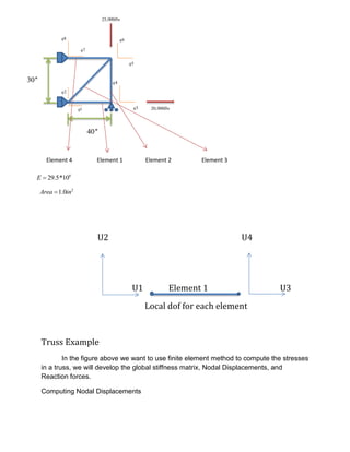
Truss Example
In the figure above we want to use finite element method to compute the stresses
in a truss, we will develop the global stiffness matrix, Nodal Displacements, and
Reaction forces.
Computing Nodal Displacements
2q
1q 3q
8q
7q
6q
5q
4q
20,000lbs
25,000lbs
40''
30''
6
29.5*10E
2
1.0Area in
2. There are 4 nodes and 4 elements making up the truss. We are going to do a two
dimensional analysis so each node is constrained to move in only the X or Y direction.
We call these directions of motion degrees of freedom or dof for short. There are 4
nodes and 8 degrees of freedom (two degrees of freedom for each node). We can
number the degrees of freedom with the formulas:
Vertical degree of freedom dof=2*node
Horizontal degree of freedom dof=2*node-1
Where node is the node number
We can locate each node by its coordinates. The table below shows the
coordinate of the nodes in the problem we are solving. We can use these coordinates to
determine the lengths and angles of the elements.
Each element can be described as extending from one node to another. This
also can be defined in a table below.
Element From
Node
To Node
1 1 2
2 3 2
3 1 3
4 4 3
From these two tables we can derive the lengths of each element and the cosine
and sine of their orientation. This is shown in the table below.
Element Length Cosine Sine
1 40 1 0
2 30 0 -1
3 50 0.8 0.6
4 40 1 0
Node X Y
1 0 0
2 40 0
3 40 30
4 0 30
3. In the formula below we can develop the stiffness matrix for an element.
2 2
2 2
2 2
2 2
. .
. .
. .
. .
Cos Cos Sin Cos Cos Sin
Cos Sin Sin Cos Sin SinAE
K
L Cos Cos Sin Cos Cos Sin
Cos Sin Sin Cos Sin Sin
This stiffness matrix is for an element. The element attaches to two nodes and
each of these nodes has two degrees of freedom. The rows and the columns of the
stiffness matrix correlate to those degrees of freedom.
Using the equation shown on top we can construct that stiffness matrix for
element 1 defined in the table above. The stiffness matrix is:
1 2 3 4
6
1
1 0 1 0 1
0 0 0 0 229.5*10
1 0 1 0 340
0 0 0 0 4
K
Element 2
6
2
0 0 0 0 5
0 1 0 1 629.5*10
0 0 0 0 330
0 1 0 1 4
K
Element 3
6
3
0.64 0.48 0.64 0.48 1
0.48 0.36 0.48 0.36 229.5*10
0.64 0.48 0.64 0.48 550
0.48 0.36 0.48 0.36 6
K
4. Element 4
6
4
1 0 1 0 7
0 0 0 0 829.5*10
1 0 1 0 540
0 0 0 0 6
K
The next step is to add the stiffness matrices for the element to create a matrix
for the entire structure. We can facilitate this by creating a common factor for Young’s
modulus and the length of the elements.
For element 1, we divide the outside by 15 and multiply each element of the
matrix by 15. Multiplying and dividing by the same number is the same as multiplying
and dividing by 1.
6
1
15 0 15 0 1
0 0 0 0 229.5*10
15 0 15 0 3600
0 0 0 0 4
K
Multiply and divide element 2 by 20.
6
2
0 0 0 0 5
0 20 0 20 629.5*10
0 0 0 0 3600
0 20 0 20 4
K
Multiply and divide element 3 by 12.
6
3
7.68 5.76 7.68 5.76 1
5.76 4.32 5.76 4.32 229.5*10
7.68 5.76 7.68 5.76 5600
5.76 4.32 5.76 4.32 6
K
5. We do the same for element 4 by multiplying and dividing it by 15.
6
4
15 0 15 0 7
0 0 0 0 829.5*10
15 0 15 0 5600
0 0 0 0 6
K
The coefficient for each stiffness matrix is the same so we can easily add the
matrices. We add the degree of freedom for each element stiffness matrix into the same
degree of freedom in the structural matrix. The resulting structural stiffness matrix is
shown below.
6
1 2 3 4 5 6 7 8
22.68 5.76 15.0 0 7.68 5.76 0 0 1
5.76 4.32 0 0 5.76 4.32 0 0 2
15.0 0 15.0 0 0 0 0 0 3
29.5*10
0 0 0 20.0 0 20.0 0 0 4
600
7.68 5.76 0 0 22.68 5.76 15.0 0 5
5.76 4.32 0 20.0 5.76 24.32 0 0 6
0 0 0 0 15.0 0 15.0 0 7
0 0 0 0 0 0 0 0 8
K
Now remembering the basic equation
*K Q F
Where K is the structural stiffness matrix, Q is the displacement of each node, and F is
the external force matrix. This result in equation below by substituting
6. 1
2
36
22.68 5.76 15.0 0 7.68 5.76 0 0
5.76 4.32 0 0 5.76 4.32 0 0
15.0 0 15.0 0 0 0 0 0
29.5*10
0 0 0 20.0 0 20.0 0 0
600
7.68 5.76 0 0 22.68 5.76 15.0 0
5.76 4.32 0 20.0 5.76 24.32 0 0
0 0 0 0 15.0 0 15.0 0
0 0 0 0 0 0 0 0
q
q
q
4
5
6
7
8
0
0
20,000
0
0
25,000
0
0
q
q
q
q
q
We have boundary conditions at the fixed supports. Our assumption is that these
joints will not move in the constrained displacements are dof 1, 2, 4, 7, and 8. The
resulting matrix is:
36
5
4
15 0 0 20,000
29.5*10
0 22.68 5.76 0
600
0 5.76 24.32 25,000
q
q
q
We can use Gaussian elimination or any number of other solution techniques to
solve the system of equations shown above. Doing so yields
3
3
3
5
3
4
27.12*10
5.65*10
22.25*10
q
q inches
q
Computing stresses
We can find the stresses by the formula below
E
Cos Sin Cos Sin q
L
We use this equation to compute the stress in each element.
8. Computing the reactions
The last step is to compute the support reactions. We need to determine the
reaction forces along dof 1, 2, 3, 7, and 8 which correspond to the fixed supports. These
are obtained by substituting Q into the original finite element equation.
R KQ F
We only need to use those rows of the structural stiffness matrix that correspond
to the fixed supports. At these supports, we are not supplying an external force so F=0.
Our equation becomes
R KQ
Or
1 3
2 6
4 3
7 3
8
0
0
22.68 5.76 15.0 0 7.68 5.76 0 0
27.12*10
5.76 4.32 0 0 5.76 4.32 0 0
029.5*10
0 0 0 20 0 20 0 0
5.65*10600
0 0 0 0 15.0 0 15.0 0
22.25*10
0 0 0 0 0 0 0 0
0
0
R
R
R
R
R
We multiply the stiffness matrix K and the deformation vector Q to get the
reactions.
They are shown in the following equation.
1
2
4
7
8
15,8333
3,126
21,879
4,167
0
R
R
R
R
R