SlideShare une entreprise Scribd logo
1  sur  18
Télécharger pour lire hors ligne
STAT9101
Term Project: Repeated Measures
Qingyang(Kevin) Liu
May 8,2017
1 Introduction
This is my last project before my graduation. I had a difficult time choosing topics from state space
model, space-time model and models with repeated measurements. Finally I decide to do the term project
about models with repeated measurements since I feel like this is the most challenge topic for me. My
only experience about linear mixed model was from STAT8004. Dr.Tang spent one course introducing linear
mixed model. Unfortunately, I was not able to learn that topic well since lacking of background/foundational
knowledge. I wish to learn a lot from this final project and actually know much more about this topic now.
2 Description of Dataset
I have spent much time finding a dataset for this project. However, most dataset for repeated measures
are either too complicated for me as a beginner to analysis or have been used as a example in textbooks.
I decide to modify a dataset, so this dataset is not only unique but also simple enough for me to show
many important components from the models I built, including but not limit to fixed effect/random effect
parameters, estimated covariance correlation matrix.
The dataset BodyWeight is from package nlme in R software. The original dataset was not equally measured
so assuming residual has AR or ARMA structure is not appropriate. The body weights of the rats (in grams)
are measured on day 1 and every seven days thereafter until day 64, with an extra measurement on day 44.
I drop the extra measurement on day 44 so now the dataset becomes equally measured.
Obs weight Time Rat Diet
1 240 1 1 1
2 250 8 1 1
3 255 15 1 1
4 260 22 1 1
5 262 29 1 1
6 258 36 1 1
7 266 43 1 1
8 265 50 1 1
9 272 57 1 1
10 278 64 1 1
11 225 1 2 1
12 230 8 2 1
13 230 15 2 1
14 232 22 2 1
15 240 29 2 1
Table 2.1: First 15 observations from modified BodyWeight
1
Table 2.1 describes the first 15 observations from modified BodyWeight.
weight: body weights of rats in grams
Time: days since the experiment began
Rat: index for rats. Range: 1 − 16
Diet: 3 types of diets.
Time (Weeks)
WeightinGrams
240250260270
1 2 3 4 5 6 7 8 9 10
Rat:1 Diet:1
225230235240245
Rat:2 Diet:1
245250255260265270
1 2 3 4 5 6 7 8 9 10
Rat:3 Diet:1
255260265270275
Rat:4 Diet:1
255260265270275280
Rat:5 Diet:1
260265270275280285
Rat:6 Diet:1
260265270275280285
Rat:7 Diet:1
250260270
Rat:8 Diet:1
420440460480500
Rat:10 Diet:2
445450455460465470
Rat:11 Diet:2
560580600620
Rat:12 Diet:2
420440460480
Rat:9 Diet:2
470490510
Rat:13 Diet:3
1 2 3 4 5 6 7 8 9 10
530540550560
Rat:14 Diet:3
520530540550
Rat:15 Diet:3
1 2 3 4 5 6 7 8 9 10
510530550570
Rat:16 Diet:3
Figure 2.1: Bodyweights of all 16 rats from first week to tenth week by 3 different diets
From Figure 2.1, we can get the conclusion that the increment of bodyweights varies by each rat, diet type.
It is interesting to find out which factor plays a more important roles in bodyweight gain and that whether
there is a difference between the effects from those three diet types.
2
3 Model Building
For analysis of repeated measures data, there are usually three different approaches, Linear Mixed Model,
MANOVA and Fixed Effect Model. In this project, I will discuss Fixed Effect Model and Linear Mixed
Model.
3.1 Fixed effect model with uncorrelated residuals
The first model I build only contains fixed effect Xβ. The residuals are identical independent normal dis-
tributed as Var(ϵ) = σ2
I and E(ϵ) = 0.
For this particular dataset, the model is
Yijk = µ + αi + γk + (αγ)ik + eijk
where
µ: interception.
αi: effect of i diet.
γk: time effect at k. (αγ)ik: diet × time interaction.
Yijk: weight in grams of rat j under idiet at time k.
eijk: residual of rat j under i diet at time k. Cov(eijk, ei′
j′
k′ ) = 0.
Time (Weeks)
Residual
−10−50
1 2 3 4 5 6 7 8 9 10
Rat:1 Diet:1
−30−28−26
Rat:2 Diet:1
−6−4−20
1 2 3 4 5 6 7 8 9 10
Rat:3 Diet:1
02468
Rat:4 Diet:1
2468
Rat:5 Diet:1
810121416
Rat:6 Diet:1
510152025
Rat:7 Diet:1
−6−20246
Rat:8 Diet:1
−45−35−25
Rat:10 Diet:2
−40−20
Rat:11 Diet:2
100105110
Rat:12 Diet:2
−46−44−42
Rat:9 Diet:2
−40−35−30−25
Rat:13 Diet:3
1 2 3 4 5 6 7 8 9 10
510152025
Rat:14 Diet:3
05101520
Rat:15 Diet:3
1 2 3 4 5 6 7 8 9 10
051015
Rat:16 Diet:3
Figure 3.1: Residuals from fixed effects model
From Figure 3.1, we can see how implausible it is to assume Cov(eijk, ei′
j′
k′ ) = 0 since residuals that follow
MVN(0, I) should fluctuate around 0 at y-axis . Next, we improve our model by assuming correlated resid-
uals.
3
Code in SAS:
PROC MIXED DATA = stat9101.Termproject;
CLASS Time Rat Diet;
MODEL weight = diet time diet*time/S RESIDUAL OUTP = out1;
RUN;
3.2 Fixed effect model with correlated residuals
The fixed effect with correlated model is
Yijk = µ + αi + γk + (αγ)ik + eijk
where
µ: interception.
αi: effect of i diet.
γk: time effect at k. (αγ)ik: diet × time interaction.
Yijk: weight in grams of rat j under idiet at time k.
eijk: residual of rat j under i diet at time k. Cov(eijk, ei′
j′
l) = 0 if either i ̸= i
′
or j ̸= j
′
. This means that
within same subject, rat,correlations between measurements based on different time lag only dependent on
the length of time interval. In this dataset, each rat will stick with same diet type. Hence, we only need to
assume
Var(eijk) = σ2
k and Cov(eijk, eijk′ ) = σkk′
We can express the vector of observations on rat j feed by diet i as Y ij = (Yij1, ..., Yjit)
′
and variance-
covariance matrix of Y as Var(Y ij) = Σ, where the element in row k and column k
′
is σkk′ . Re-express
variance-covariance matrix of Y as Var(Y ) = I ⊗ Σ. For this dataset, each rat is considered to have co-
variance matrix Σ. In SAS Mixed procedure, the form of Σ can be specified through REPEATED statement.
There are totally 17 types of covariance structures we can choose from REPEATED statement. I will
build models only using some common covariance structures like compounds symmetry, unstructured,
AR(1),Heterogeneous AR(1), Toeplitz,Heterogeneous Toeplitz and ARMA(1,1).
Code in SAS:
PROC MIXED DATA = stat9101.Termproject;
CLASS time rat diet;
MODEL weight = diet time diet*time/S RESIDUAL OUTP = out1;
RUN;
3.2.1 Fixed effect model with unstructured covariance matrix
We use ML to estimate parameters. Note that REML is the default algorithm by SAS Mixed Procedur.
However, later on we need to do log-likelihood ratio test for model selection, so we choose ML instead of
REML.
ˆΣ =
















1159.96 1112.89 1045.90 1105.43 1104.34 1103.44 1065.59 1106.88 1033.75 1038.75
1112.89 1091.80 1034.77 1095.55 1099.77 1098.98 1066.02 1107.11 1039.22 1039.61
1045.90 1034.77 1000.98 1053.79 1059.96 1057.73 1029.73 1069.14 1006.56 1011.25
1105.43 1095.55 1053.79 1130.60 1127.87 1128.98 1100.16 1146.02 1082.13 1078.72
1104.34 1099.77 1059.96 1127.87 1139.09 1143.81 1118.96 1161.00 1101.75 1103.50
1103.44 1098.98 1057.73 1128.98 1143.81 1158.47 1134.30 1177.69 1118.22 1123.77
1065.59 1066.02 1029.73 1100.16 1118.96 1134.30 1121.10 1160.33 1108.88 1114.88
1106.88 1107.11 1069.14 1146.02 1161.00 1177.69 1160.33 1211.34 1151.59 1162.52
1033.75 1039.22 1006.56 1082.13 1101.75 1118.22 1108.88 1151.59 1107.19 1117.91
1038.75 1039.61 1011.25 1078.72 1103.50 1123.77 1114.88 1162.52 1117.91 1153.33
















4
Note that covariance matrix is symmetric. ˆΣ = ˆΣ
t
The unstructured covariance is the most complicated structure, which contains 11 × 10/2 = 55 parame-
ters. The variances on the diagonal of this covariance matrix are the estimated variances of measures from
week1 to week 10. The covariance σi,k measures the covariance between week i and week k. For example,
σ1,2 = 1112.89 is covariance between measures week 1 and week 2.
The correlation matrix of residual, which equals to corr(ϵ) = (diag(Σ))
− 1
2
Σ (diag(Σ))
− 1
2
, is shown below.
corr(ϵ) =
















1.000 0.989 0.971 0.965 0.961 0.952 0.934 0.934 0.912 0.898
0.989 1.000 0.990 0.986 0.986 0.977 0.964 0.963 0.945 0.927
0.971 0.990 1.000 0.991 0.993 0.982 0.972 0.971 0.956 0.941
0.965 0.986 0.991 1.000 0.994 0.987 0.977 0.979 0.967 0.945
0.961 0.986 0.993 0.994 1.000 0.996 0.990 0.988 0.981 0.963
0.952 0.977 0.982 0.987 0.996 1.000 0.995 0.994 0.987 0.972
0.934 0.964 0.972 0.977 0.990 0.995 1.000 0.996 0.995 0.981
0.934 0.963 0.971 0.979 0.988 0.994 0.996 1.000 0.994 0.984
0.912 0.945 0.956 0.967 0.981 0.987 0.995 0.994 1.000 0.989
0.898 0.927 0.941 0.945 0.963 0.972 0.981 0.984 0.989 1.000
















For example the correlation for residual of weight measures between week1 and week2, can be found in the
first row, second column of the correlation matrix above. We can see that the longer of the time lags spans,
the smaller correlation is. In other words, residuals of weight measurement at week1 has weaker influence
on residuals of weight measurement at week3 or on following weeks than residuals of weight measurement at
week2. This makes logical sense. We can use this property of decaying correlation to do model comparison.
We will also do model comparison by using information criterion and log-likelihood test. The information
criterion could be found in table 3.1
Fit Statistics
-2 Log Likelihood 879
AIC (Smaller is Better) 1049
AICC (Smaller is Better) 1246.6
BIC (Smaller is Better) 1114.7
Table 3.1: Information criterion of fixed effect model with unstructured covariance matrix
Null Model Likelihood Ratio Test
DF Chi-Square Pr >ChiSq
54 699.47 <.0001
Table 3.2: Null Model Likelihood Ratio Test with unstructured covariance matrix
Table 3.2 shows the results of null model likelihood ratio test. The null hypothesis is that the null model,
which is fixed effect model with uncorrelated residual,Σ = σ2
I, fits as good as the model with the specified
covariance structure. The alternative hypothesis is that the model with more parameters fit better than the
null model does. The degree of freedom,54 = 55 − 1, is determined by the difference between the number
of parameters of null model and model with more parameters. Since the p-value is smaller than 0.0001, we
confirm the conclusion we get in section 3.1, fixed effect model with uncorrelated residuals is inadequate.
5
Type 3 Tests of Fixed Effects
Effect Num DF Den DF F Value Pr >F
Diet 2 13 107.78 <.0001
Time 9 13 66.16 <.0001
Time*Diet 18 13 19.76 <.0001
Table 3.3: Tests of Fixed Effects with unstructured covariance matrix
From the result of table 3.3, we have that under fixed effects model with unstructured covariance, all three
fixed effect, diet, time and interaction between diet and time have significant effect on rats’ bodyweight. We
still need to try other models with different covariance structure and recheck our conclusion here.
Code in SAS:
PROC MIXED DATA = stat9101.Termproject METHOD = ML;
CLASS time rat diet;
MODEL weight = diet time diet*time/S RESIDUAL OUTP = out2;
REPEATED time / SUBJECT = rat(diet) TYPE = UN R RCORR;
RUN;
3.2.2 Fixed effect model with compound symmetry covariance matrix: a inadequate model
The compound symmetry structure:
Σ =







σ2
+ σ1 σ1 σ1 . . . σ1
σ2
+ σ1 σ1 . . . σ1
...
...
...
σ2
+ σ1 σ1
σ2
+ σ1







There are two parameters, σ and σ1 for the compound symmetry structure.
Covariance Parameter Estimates
Cov Parm Subject Estimate
CS Rat(Diet) 1094.42
Residual 32.9609
Table 3.4: Covariance Parameter Estimates for compound symmetry structure
From table 3.4 we have σ1 = 1094.42 and σ2
= 32.9609. We have estimated covariance matrix of residuals
like following:
ˆΣ =
















1127.39 1094.42 1094.42 1094.42 1094.42 1094.42 1094.42 1094.42 1094.42 1094.42
1094.42 1127.39 1094.42 1094.42 1094.42 1094.42 1094.42 1094.42 1094.42 1094.42
1094.42 1094.42 1127.39 1094.42 1094.42 1094.42 1094.42 1094.42 1094.42 1094.42
1094.42 1094.42 1094.42 1127.39 1094.42 1094.42 1094.42 1094.42 1094.42 1094.42
1094.42 1094.42 1094.42 1094.42 1127.39 1094.42 1094.42 1094.42 1094.42 1094.42
1094.42 1094.42 1094.42 1094.42 1094.42 1127.39 1094.42 1094.42 1094.42 1094.42
1094.42 1094.42 1094.42 1094.42 1094.42 1094.42 1127.39 1094.42 1094.42 1094.42
1094.42 1094.42 1094.42 1094.42 1094.42 1094.42 1094.42 1127.39 1094.42 1094.42
1094.42 1094.42 1094.42 1094.42 1094.42 1094.42 1094.42 1094.42 1127.39 1094.42
1094.42 1094.42 1094.42 1094.42 1094.42 1094.42 1094.42 1094.42 1094.42 1127.39
















6
We can hand check the first number in estimated covariance matrix: 1127.39 ≈ 1094.42 + 32.9609
Correlation matrix as:
corr(ϵ) =
















1.0000 0.9708 0.9708 0.9708 0.9708 0.9708 0.9708 0.9708 0.9708 0.9708
0.9708 1.0000 0.9708 0.9708 0.9708 0.9708 0.9708 0.9708 0.9708 0.9708
0.9708 0.9708 1.0000 0.9708 0.9708 0.9708 0.9708 0.9708 0.9708 0.9708
0.9708 0.9708 0.9708 1.0000 0.9708 0.9708 0.9708 0.9708 0.9708 0.9708
0.9708 0.9708 0.9708 0.9708 1.0000 0.9708 0.9708 0.9708 0.9708 0.9708
0.9708 0.9708 0.9708 0.9708 0.9708 1.0000 0.9708 0.9708 0.9708 0.9708
0.9708 0.9708 0.9708 0.9708 0.9708 0.9708 1.0000 0.9708 0.9708 0.9708
0.9708 0.9708 0.9708 0.9708 0.9708 0.9708 0.9708 1.0000 0.9708 0.9708
0.9708 0.9708 0.9708 0.9708 0.9708 0.9708 0.9708 0.9708 1.0000 0.9708
0.9708 0.9708 0.9708 0.9708 0.9708 0.9708 0.9708 0.9708 0.9708 1.0000
















where 0.9708 = 1094.42/1127.39
From estimated correlation matrix, we can see that compound symmetry structure may be inappropriate
for this dataset. Because the correlation of weight measures between different time lags does not vary. We
confirm this guess using following methods.
Fit Statistics
-2 Log Likelihood 1106.2
AIC (Smaller is Better) 1170.2
AICC (Smaller is Better) 1186.9
BIC (Smaller is Better) 1195.0
Table 3.5: Information Criterion for fixed effects model with compound symmetry structure
By comparing table 3.5 and table 3.1, we find fixed effects model with compound symmetry structure has
larger information criterion. By using log-likelihood test, we have p-value < 0.001 where χ2
= 1106.2−879 =
227.2, df = 55 − 2. Based on the result of comparing information criterion and log-likelihood test, we get
the conclusion that model with unstructured covariance are is more adequate than model with compound
symmetry structure.
Type 3 Tests of Fixed Effects
Effect Num DF Den DF F Value Pr >F
Diet 2 13 107.78 <.0001
Time 9 117 90.19 <.0001
Time*Diet 18 117 8.27 <.0001
Table 3.6: Type 3 Tests of Fixed Effects with compound symmetry structure
According to table 3.6, our conclusion from section 3.2.1 remains the same, that all three fixed effect, diet,
time and interaction between diet and time have significant effect on rats’ bodyweight.
Code in R
> pchisq(227.2,df = 55-2, lower.tail = F)
[1] 1.946558e-23
7
Code in SAS
PROC MIXED DATA = stat9101.Termproject METHOD = ML;
CLASS time rat diet;
MODEL weight = diet time diet*time/S RESIDUAL OUTP = out2;
REPEATED time / SUBJECT = rat(diet) TYPE = CS R RCORR;
RUN;
3.2.3 Fixed effect model with AR(1) structure and other common structures
The AR(1) structure:
Σ = σ2




1.0 ρ ρ2
ρ3
1.0 ρ ρ2
1.0 ρ
1.0




There are two parameters of this covariance structure.
Covariance Parameter Estimates
Cov Parm Subject Estimate
AR(1) Rat(Diet) 0.9923
Residual 1154.53
Table 3.7: Covariance Parameter Estimates for AR(1) structure
From table 3.7, we have σ2
= 1154.53, ρ = 0.9923 and the estimated covariance matrix as
ˆΣ =
















1154.53 1145.65 1136.83 1128.08 1119.40 1110.79 1102.24 1093.75 1085.34 1076.98
1145.65 1154.53 1145.65 1136.83 1128.08 1119.40 1110.79 1102.24 1093.75 1085.34
1136.83 1145.65 1154.53 1145.65 1136.83 1128.08 1119.40 1110.79 1102.24 1093.75
1128.08 1136.83 1145.65 1154.53 1145.65 1136.83 1128.08 1119.40 1110.79 1102.24
1119.40 1128.08 1136.83 1145.65 1154.53 1145.65 1136.83 1128.08 1119.40 1110.79
1110.79 1119.40 1128.08 1136.83 1145.65 1154.53 1145.65 1136.83 1128.08 1119.40
1102.24 1110.79 1119.40 1128.08 1136.83 1145.65 1154.53 1145.65 1136.83 1128.08
1093.75 1102.24 1110.79 1119.40 1128.08 1136.83 1145.65 1154.53 1145.65 1136.83
1085.34 1093.75 1102.24 1110.79 1119.40 1128.08 1136.83 1145.65 1154.53 1145.65
1076.98 1085.34 1093.75 1102.24 1110.79 1119.40 1128.08 1136.83 1145.65 1154.53
















Estimated correlation matrix as
corr(ϵ) =
















1.000 0.992 0.985 0.977 0.970 0.962 0.955 0.947 0.940 0.933
0.992 1.000 0.992 0.985 0.977 0.970 0.962 0.955 0.947 0.940
0.985 0.992 1.000 0.992 0.985 0.977 0.970 0.962 0.955 0.947
0.977 0.985 0.992 1.000 0.992 0.985 0.977 0.970 0.962 0.955
0.970 0.977 0.985 0.992 1.000 0.992 0.985 0.977 0.970 0.962
0.962 0.970 0.977 0.985 0.992 1.000 0.992 0.985 0.977 0.970
0.955 0.962 0.970 0.977 0.985 0.992 1.000 0.992 0.985 0.977
0.947 0.955 0.962 0.970 0.977 0.985 0.992 1.000 0.992 0.985
0.940 0.947 0.955 0.962 0.970 0.977 0.985 0.992 1.000 0.992
0.933 0.940 0.947 0.955 0.962 0.970 0.977 0.985 0.992 1.000
















Now the correlation between different time lags begins to decays.
It would be very tedious to show the estimated covariance and correlation matrix of all 7 models. I will use
information criterion as a model selection tool to choose the best model.
8
Fit Statistics-AR(1) Fit Statistics-ARH(1) Fit Statistics-ARMA(1,1)
-2 Log Likelihood 980.7 -2 Log Likelihood 970 -2 Log Likelihood 979.5
AIC (Smaller is Better) 1044.7 AIC (Smaller is Better) 1052 AIC (Smaller is Better) 1045.5
AICC (Smaller is Better) 1061.3 AICC (Smaller is Better) 1081.2 AICC (Smaller is Better) 1063.3
BIC (Smaller is Better) 1069.4 BIC (Smaller is Better) 1083.7 BIC (Smaller is Better) 1071.0
Fit Statistics-Unstructured Fit Statistics-Toeplitz Fit Statistics-Heterogeneous Toeplitz
-2 Log Likelihood 879.0 -2 Log Likelihood 967.0 -2 Log Likelihood 954.3
AIC (Smaller is Better) 1049.0 AIC (Smaller is Better) 1047.0 AIC (Smaller is Better) 1052.3
AICC (Smaller is Better) 1246.6 AICC (Smaller is Better) 1074.5 AICC (Smaller is Better) 1096.8
BIC (Smaller is Better) 1114.7 BIC (Smaller is Better) 1077.9 BIC (Smaller is Better) 1090.1
Table 3.8: Information Criterion
Note that the information criterion for compound symmetry is not in table 3.8 but in table 3.5. Overall
fixed effect model with AR(1) structure is indeed the best model between these 7 models.
Type 3 Tests of Fixed Effects
Effect Num DF Den DF F Value Pr >F
Diet 2 13 105.10 <.0001
Time 9 117 27.71 <.0001
Time*Diet 18 117 5.69 <.0001
Table 3.9: Test of Fixed Effects - AR(1) structure
From table 3.9, we have the conclusion that all three fixed effect, diet, time and interaction between diet
and time have significant effect on rats’ bodyweight.
From table 3.10, the difference between effects from diet1 and diet3 are significant all the time, so is the
difference between effect from diet1 and diet2.The difference between diet2 and diet3 is significant until time
lag 8(week2).Table 3.10 was created through SAS PROC GLIMMIX. The results from SAS PROC GLIMMIX and
SAS PROC MIXED is negligible.
From table 3.11, we have that the bodyweight of rats by diet1 increases faster than other diet types since
the estimated parameters for interaction between time and diet1 are positive and significantly different from
zero all the time. The intercept of fixed effect from diet2 is not significant since p-value is 0.21. The time
effects are significant from first week to last week. All rats will gain weights while time lag increases. The
interaction between time and diet2 becomes insignificant after time lag8(week2). This finding is as same as
what we have from table 3.10.
Code in SAS:
proc mixed data = stat9101.Termproject;
class Time Rat Diet;
model weight = diet time diet*time/S;
repeated time/ subject = rat type = AR(1) R;
run;
proc glimmix data = stat9101.Termproject outdesign = design1;
class Time Rat Diet;
model weight = diet time diet*time;
random time/ subject = rat residual type = AR(1) S G;
run;
proc mixed data = stat9101.Termproject;
class Time Rat Diet;
9
model weight = diet time diet*time/S;
repeated time/ subject = rat type = AR(1) R;
random Rat/G S;
run;
proc glimmix data = stat9101.Termproject outdesign = design2;
class Time Rat Diet;
model weight = diet time diet*time/S;
random time/ subject = rat residual type = AR(1);
random Rat/G S;
run;
/*Fixed Model*/
PROC MIXED DATA = stat9101.Termproject;
CLASS time rat diet;
MODEL weight = diet time diet*time/S RESIDUAL OUTP = out1;
RUN;
/*Fixed Model with unstrcucred matrix*/
PROC MIXED DATA = stat9101.Termproject METHOD = ML;
CLASS time rat diet;
MODEL weight = diet time diet*time/S RESIDUAL OUTP = out2;
REPEATED time / SUBJECT = rat(diet) TYPE = UN R RCORR;
RUN;
/*Fixed Model with compound symmetry matrix*/
PROC MIXED DATA = stat9101.Termproject METHOD = ML;
CLASS time rat diet;
MODEL weight = diet time diet*time/S RESIDUAL OUTP = out2;
REPEATED time / SUBJECT = rat(diet) TYPE = CS R RCORR;
RUN;
/*Fixed Model with AR(1)*/
PROC MIXED DATA = stat9101.Termproject METHOD = ML;
CLASS time rat diet;
MODEL weight = diet time diet*time/S RESIDUAL OUTP = out1;
REPEATED time / SUBJECT = rat(diet) TYPE = AR(1) R RCORR;
RUN;
/*Fixed Model with ARH(1)*/
PROC MIXED DATA = stat9101.Termproject METHOD = ML;
CLASS time rat diet;
MODEL weight = diet time diet*time/S RESIDUAL OUTP = out1;
REPEATED time / SUBJECT = rat(diet) TYPE = ARH(1) R RCORR;
RUN;
/*Fixed Model with Toeplitz*/
PROC MIXED DATA = stat9101.Termproject METHOD = ML;
CLASS time rat diet;
MODEL weight = diet time diet*time/S RESIDUAL OUTP = out1;
REPEATED time / SUBJECT = rat(diet) TYPE = TOEP R RCORR;
RUN;
/*Fixed Model with Heterogeneous Toeplitz*/
PROC MIXED DATA = stat9101.Termproject METHOD = ML;
CLASS time rat diet;
MODEL weight = diet time diet*time/S RESIDUAL OUTP = out1;
REPEATED time / SUBJECT = rat(diet) TYPE = TOEPH R RCORR;
RUN;
/*Fixed Model with ARMA(1,1)*/
PROC MIXED DATA = stat9101.Termproject METHOD = ML;
CLASS time rat diet;
10
MODEL weight = diet time diet*time/S RESIDUAL OUTP = out1;
REPEATED time / SUBJECT = rat(diet) TYPE = ARMA(1,1) R RCORR;
RUN;
/*SIMPLE EFFECT COMPARISON*/
PROC GLIMMIX DATA = stat9101.Termproject NOREML OUTDESIGN = OUT1;
CLASS time(REF = FIRST) rat diet(REF = FIRST);
MODEL weight = diet time diet*time/S;
RANDOM _RESIDUAL_/ TYPE = AR(1) SUBJECT = rat(diet);
RUN;
Simple Effect Comparisons of Time*Diet Least Squares Means By Time
Simple Effect Level Diet _Diet Estimate Standard Error DF t Value Pr >|t|
Time 1 1 2 -203.13 20.81 117.00 -9.76 <.0001
Time 1 1 3 -258.13 20.81 117.00 -12.41 <.0001
Time 1 2 3 -55.00 24.03 117.00 -2.29 0.0200
Time 8 1 2 -205.00 20.81 117.00 -9.85 <.0001
Time 8 1 3 -251.25 20.81 117.00 -12.08 <.0001
Time 8 2 3 -46.25 24.03 117.00 -1.92 0.0600
Time 15 1 2 -213.13 20.81 117.00 -10.24 <.0001
Time 15 1 3 -259.38 20.81 117.00 -12.47 <.0001
Time 15 2 3 -46.25 24.03 117.00 -1.92 0.0600
Time 22 1 2 -213.13 20.81 117.00 -10.24 <.0001
Time 22 1 3 -256.38 20.81 117.00 -12.32 <.0001
Time 22 2 3 -43.25 24.03 117.00 -1.80 0.0700
Time 29 1 2 -218.13 20.81 117.00 -10.48 <.0001
Time 29 1 3 -259.13 20.81 117.00 -12.45 <.0001
Time 29 2 3 -41.00 24.03 117.00 -1.71 0.0900
Time 36 1 2 -223.75 20.81 117.00 -10.75 <.0001
Time 36 1 3 -264.25 20.81 117.00 -12.70 <.0001
Time 36 2 3 -40.50 24.03 117.00 -1.69 0.0900
Time 43 1 2 -219.12 20.81 117.00 -10.53 <.0001
Time 43 1 3 -255.37 20.81 117.00 -12.27 <.0001
Time 43 2 3 -36.25 24.03 117.00 -1.51 0.1300
Time 50 1 2 -231.75 20.81 117.00 -11.14 <.0001
Time 50 1 3 -268.75 20.81 117.00 -12.92 <.0001
Time 50 2 3 -37.00 24.03 117.00 -1.54 0.1300
Time 57 1 2 -237.50 20.81 117.00 -11.41 <.0001
Time 57 1 3 -271.00 20.81 117.00 -13.02 <.0001
Time 57 2 3 -33.50 24.03 117.00 -1.39 0.1700
Time 64 1 2 -244.75 20.81 117.00 -11.76 <.0001
Time 64 1 3 -276.50 20.81 117.00 -13.29 <.0001
Time 64 2 3 -31.75 24.03 117.00 -1.32 0.1900
Table 3.10: Simple Effect Comparisons of Time*Diet Least Squares Means By Time by PROC GLIMMIX
11
Solution for Fixed Effects
Effect Time Diet Estimate Standard Error DF t Value Pr >|t|
Intercept 550.25 16.99 13.00 32.39 <.0001
Diet 1 -276.50 20.81 13.00 -13.29 <.0001
Diet 2 -31.75 24.03 13.00 -1.32 0.21
Diet 3 0.00 . . . .
Time 1 -41.50 6.23 117.00 -6.66 <.0001
Time 8 -44.00 5.88 117.00 -7.48 <.0001
Time 15 -36.50 5.51 117.00 -6.62 <.0001
Time 22 -32.00 5.11 117.00 -6.26 <.0001
Time 29 -26.50 4.68 117.00 -5.67 <.0001
Time 36 -21.00 4.19 117.00 -5.01 <.0001
Time 43 -27.50 3.64 117.00 -7.56 <.0001
Time 50 -12.00 2.98 117.00 -4.03 <.0001
Time 57 -7.75 2.11 117.00 -3.68 0.00
Time 64 0.00 . . . .
Time*Diet 1 1 18.38 7.63 117.00 2.41 0.02
Time*Diet 1 2 -23.25 8.81 117.00 -2.64 0.01
Time*Diet 1 3 0.00 . . . .
Time*Diet 8 1 25.25 7.20 117.00 3.51 0.00
Time*Diet 8 2 -14.50 8.32 117.00 -1.74 0.08
Time*Diet 8 3 0.00 . . . .
Time*Diet 15 1 17.13 6.75 117.00 2.54 0.01
Time*Diet 15 2 -14.50 7.80 117.00 -1.86 0.07
Time*Diet 15 3 0.00 . . . .
Time*Diet 22 1 20.13 6.26 117.00 3.21 0.00
Time*Diet 22 2 -11.50 7.23 117.00 -1.59 0.11
Time*Diet 22 3 0.00 . . . .
Time*Diet 29 1 17.38 5.73 117.00 3.03 0.00
Time*Diet 29 2 -9.25 6.61 117.00 -1.40 0.16
Time*Diet 29 3 0.00 . . . .
Time*Diet 36 1 12.25 5.13 117.00 2.39 0.02
Time*Diet 36 2 -8.75 5.93 117.00 -1.48 0.14
Time*Diet 36 3 0.00 . . . .
Time*Diet 43 1 21.13 4.45 117.00 4.74 <.0001
Time*Diet 43 2 -4.50 5.14 117.00 -0.87 0.38
Time*Diet 43 3 0.00 . . . .
Time*Diet 50 1 7.75 3.64 117.00 2.13 0.04
Time*Diet 50 2 -5.25 4.21 117.00 -1.25 0.21
Time*Diet 50 3 0.00 . . . .
Time*Diet 57 1 5.50 2.58 117.00 2.13 0.04
Time*Diet 57 2 -1.75 2.98 117.00 -0.59 0.56
Time*Diet 57 3 0.00 . . . .
Time*Diet 64 1 0.00 . . . .
Time*Diet 64 2 0.00 . . . .
Time*Diet 64 3 0.00 . . . .
Table 3.11: Fixed Effect analysis-AR(1)
12
3.3 Linear Mixed Model-with fixed and random effect - inappropriate model
It is very nature to consider the subject of this experiment, rats, as random effect. Now we will have another
covariance matrix G.
The linear mixed model is:
y = Xβ + Zγ + ϵ
where
(
γ
ϵ
)
∼ N
((
0
0
) (
G 0
0 R
))
Assuming ϵ has AR(1) structure, we get ˆG matrix and ˆR matrix below by MIVQUE0 method instead
of REML or MLE. SAS software can’t estimate G matrix by REML or ML method. The SAS console
shows Estimated G matrix is not positive definite. I don’t know much about the difference between
MIVQUE0 and MLE or REMLE(I do know the difference between MLE and REMLE). According to SAS
MIXED PROCEDURE MANUAL 14.1, MIVQUE0 method is a non-iterative method and in fact estimates
starting values for the ML and REMLE methods. MIVQUE0 method turns out to be the only method that
esitmates ˆR matrix successfully.
ˆR =
















46.975 32.040 21.853 14.905 10.166 6.934 4.729 3.226 2.200 1.501
32.040 46.975 32.040 21.853 14.905 10.166 6.934 4.729 3.226 2.200
21.853 32.040 46.975 32.040 21.853 14.905 10.166 6.934 4.729 3.226
14.905 21.853 32.040 46.975 32.040 21.853 14.905 10.166 6.934 4.729
10.166 14.905 21.853 32.040 46.975 32.040 21.853 14.905 10.166 6.934
6.934 10.166 14.905 21.853 32.040 46.975 32.040 21.853 14.905 10.166
4.729 6.934 10.166 14.905 21.853 32.040 46.975 32.040 21.853 14.905
3.226 4.729 6.934 10.166 14.905 21.853 32.040 46.975 32.040 21.853
2.200 3.226 4.729 6.934 10.166 14.905 21.853 32.040 46.975 32.040
1.501 2.200 3.226 4.729 6.934 10.166 14.905 21.853 32.040 46.975
















Estimated G Matrix
Row Effect Rat Diet Col1 Col2 Col3 Col4 Col5 Col6 Col7 Col8 Col9 Col10 Col11 Col12 Col13 Col14 Col15 Col16
1 Rat(Diet) 1 1 1340.58
2 Rat(Diet) 2 1 1340.58
3 Rat(Diet) 3 1 1340.58
4 Rat(Diet) 4 1 1340.58
5 Rat(Diet) 5 1 1340.58
6 Rat(Diet) 6 1 1340.58
7 Rat(Diet) 7 1 1340.58
8 Rat(Diet) 8 1 1340.58
9 Rat(Diet) 9 2 1340.58
10 Rat(Diet) 10 2 1340.58
11 Rat(Diet) 11 2 1340.58
12 Rat(Diet) 12 2 1340.58
13 Rat(Diet) 13 3 1340.58
14 Rat(Diet) 14 3 1340.58
15 Rat(Diet) 15 3 1340.58
16 Rat(Diet) 16 3 1340.58
Table 3.12: Estimated ˆG matrix
The ˆG is shown in table 3.12, not in matrix form since the first four columns explains the meaning of this
matrix very well. This diagonal form matrix implies that covariance between different rats is zero. It plau-
sible to assume that effects on different rats are independent.
From table 3.13, we have that adding random effect is not necessary for this dataset. The model with random
effects have 1 more parameter for ˆG and 16 more parameters for random slopes. Adding more parameters
13
without improving the model increases information criterion. We can not compare table 3.8 and table 3.13
since they are created by ML and MIVQUE0 methods respectively.
Fit Statistics-no random effects Fit Statistics-with random effect
-2 Res Log Likelihood 877.5 -2 Res Log Likelihood 891.6
AIC (Smaller is Better) 881.5 AIC (Smaller is Better) 897.6
AICC (Smaller is Better) 881.6 AICC (Smaller is Better) 897.8
BIC (Smaller is Better) 883.0 BIC (Smaller is Better) 900.0
Table 3.13: Information criterion-by MIVQUE0 method
From table 3.14, we have that based on linear mixed model (even though it is not necessary to add random
effect),all three fixed effect, diet, time and interaction between diet and time have significant effect on rats’
bodyweight.
Type 3 Tests of Fixed Effects
Effect Num DF Den DF F Value Pr >F
Diet 2 13 87.04 <.0001
Time 9 117 37.96 <.0001
Time*Diet 18 117 5 <.0001
Table 3.14: Fixed effect analysis from linear mixed model
Solution for Random Effects
Effect Rat Diet Estimate Std Err Pred DF t Value Pr >|t|
Rat(Diet) 1 1 -2.853 13.513 117.000 -0.210 0.833
Rat(Diet) 2 1 -26.269 13.513 117.000 -1.940 0.054
Rat(Diet) 3 1 -4.206 13.513 117.000 -0.310 0.756
Rat(Diet) 4 1 3.397 13.513 117.000 0.250 0.802
Rat(Diet) 5 1 5.538 13.513 117.000 0.410 0.683
Rat(Diet) 6 1 10.089 13.513 117.000 0.750 0.457
Rat(Diet) 7 1 13.170 13.513 117.000 0.970 0.332
Rat(Diet) 8 1 1.135 13.513 117.000 0.080 0.933
Rat(Diet) 9 2 -42.881 18.655 117.000 -2.300 0.023
Rat(Diet) 10 2 -33.148 18.655 117.000 -1.780 0.078
Rat(Diet) 11 2 -28.221 18.655 117.000 -1.510 0.133
Rat(Diet) 12 2 104.250 18.655 117.000 5.590 <.0001
Rat(Diet) 13 3 -32.678 18.655 117.000 -1.750 0.082
Rat(Diet) 14 3 13.148 18.655 117.000 0.700 0.482
Rat(Diet) 15 3 11.299 18.655 117.000 0.610 0.546
Rat(Diet) 16 3 8.231 18.655 117.000 0.440 0.660
Table 3.15: Solution for Random Effects
14
Solution for Fixed Effects
Effect Time Diet Estimate Standard Error DF t Value Pr >|t|
Intercept 550.25 18.6249 13 29.54 <.0001
Diet 1 -276.5 22.8108 13 -12.12 <.0001
Diet 2 -31.75 26.3396 13 -1.21 0.2495
Diet 3 0 . . . .
Time 1 -41.5 4.7684 117 -8.7 <.0001
Time 8 -44 4.7316 117 -9.3 <.0001
Time 15 -36.5 4.6771 117 -7.8 <.0001
Time 22 -32 4.596 117 -6.96 <.0001
Time 29 -26.5 4.4745 117 -5.92 <.0001
Time 36 -21 4.2901 117 -4.9 <.0001
Time 43 -27.5 4.0044 117 -6.87 <.0001
Time 50 -12 3.5442 117 -3.39 0.001
Time 57 -7.75 2.7327 117 -2.84 0.0054
Time 64 0 . . . .
Time*Diet 1 1 18.375 5.84 117 3.15 0.0021
Time*Diet 1 2 -23.25 6.7435 117 -3.45 0.0008
Time*Diet 1 3 0 . . . .
Time*Diet 8 1 25.25 5.7949 117 4.36 <.0001
Time*Diet 8 2 -14.5 6.6914 117 -2.17 0.0323
Time*Diet 8 3 0 . . . .
Time*Diet 15 1 17.125 5.7282 117 2.99 0.0034
Time*Diet 15 2 -14.5 6.6143 117 -2.19 0.0303
Time*Diet 15 3 0 . . . .
Time*Diet 22 1 20.125 5.6289 117 3.58 0.0005
Time*Diet 22 2 -11.5 6.4997 117 -1.77 0.0794
Time*Diet 22 3 0 . . . .
Time*Diet 29 1 17.375 5.4801 117 3.17 0.0019
Time*Diet 29 2 -9.25 6.3278 117 -1.46 0.1465
Time*Diet 29 3 0 . . . .
Time*Diet 36 1 12.25 5.2542 117 2.33 0.0214
Time*Diet 36 2 -8.75 6.0671 117 -1.44 0.1519
Time*Diet 36 3 0 . . . .
Time*Diet 43 1 21.125 4.9044 117 4.31 <.0001
Time*Diet 43 2 -4.5 5.6631 117 -0.79 0.4284
Time*Diet 43 3 0 . . . .
Time*Diet 50 1 7.75 4.3407 117 1.79 0.0768
Time*Diet 50 2 -5.25 5.0122 117 -1.05 0.2971
Time*Diet 50 3 0 . . . .
Time*Diet 57 1 5.5 3.3469 117 1.64 0.103
Time*Diet 57 2 -1.75 3.8647 117 -0.45 0.6515
Time*Diet 57 3 0 . . . .
Time*Diet 64 1 0 . . . .
Time*Diet 64 2 0 . . . .
Time*Diet 64 3 0 . . . .
Table 3.16: Solution for Fixed Effects
15
The estimated ˆβ and ˆγ could be found in table 3.16 and table 3.15 respectively. It is easy to find out that
many estimated parameters in table 3.15 are not significantly different from 0, this confirms the conclusion
that adding random effect is not nessccary for this dataset.
Code in SAS:
/*RANDOM EFFECT MODEL*/
PROC MIXED DATA = stat9101.Termproject METHOD = MIVQUE0;
CLASS time rat diet;
MODEL weight = diet time diet*time/S RESIDUAL OUTP = out1;
REPEATED time / SUBJECT = rat(diet) TYPE = AR(1) R RCORR;
RANDOM rat(diet)/S G;
RUN;
/*FIXED EEFECT MODEL*/
PROC MIXED DATA = stat9101.Termproject METHOD = MIVQUE0;
CLASS time rat diet;
MODEL weight = diet time diet*time/S RESIDUAL OUTP = out1;
REPEATED time / SUBJECT = rat(diet) TYPE = AR(1) R RCORR;
RUN;
16
4 Influence Analysis of Fixed effect model with AR(1) structure
1 2 3 4 5 6 7 8 9 10 11 12 13 14 15 16
Deleted Rat
0
2
4
6
8
10
Distance
Likelihood Distance
Influence Statistics for Fixed Effects
1 2 3 4 5 6 7 8 9 10 11 12 13 14 15 16
Deleted Rat
0
10
20
30
40
COVRATIO
1 2 3 4 5 6 7 8 9 10 11 12 13 14 15 16
0.00
0.05
0.10
0.15
0.20
0.25
Cook'sD
Figure 4.1: Influence analysis figures
The main purpose of analysis of repeated measures data is usually to study the influence of cluster(rats)
by checking ANOVA table of fixed effect like table 3.14, rather than the influence of individual observa-
tions. However, sometimes unfitted observations or outliers show us some important informations we did
not expect. Figure 4.1 contains three sub-figures, likelihood distance, Cook’s Distance and COVRATIO.
Likelihood distance and Cook’ distance acutally have exactly same trend. This shows us that fixed effect
model with AR(1) structure does not fit rat 12(diet2), 15(diet3) and 16(diet3) very well. COVRATIO shows
us that rat 9(diet2) has the most significant influence on covariance estimation. It is important to inform
other scientists to check those rats. Other scientists may find important facts hide in those data.
Table 4.1 contains the data for figure 4.1. The column, number of observations in level, means that each rat
has been measured 10 times.
17
Influence Diagnostics for Levels of Rat
Rat Number of Observations in Level Cook’s D COVRATIO Likelihood Distance
1 10 0.05208 3.149 1.575
2 10 0.05759 2.493 1.768
3 10 0.01964 12.037 0.684
4 10 0.03734 5.835 1.121
5 10 0.02827 8.475 0.882
6 10 0.03527 6.357 1.063
7 10 0.08014 0.939 2.695
8 10 0.04198 4.813 1.254
9 10 0.06899 37.546 2.068
10 10 0.13364 11.805 4.079
11 10 0.16226 6.971 5.100
12 10 0.21294 2.679 7.129
13 10 0.13539 11.434 4.139
14 10 0.18676 4.408 6.044
15 10 0.27533 0.790 10.054
16 10 0.23598 1.717 8.151
Table 4.1: Influence diagnostics for each rat
Code in SAS:
/*INFLUENCE ANALYSIS*/
PROC MIXED DATA = stat9101.Termproject METHOD = ML;
CLASS time rat diet;
MODEL weight = diet time diet*time/S RESIDUAL OUTP = out1 INFLUENCE(EFFECT = rat);
REPEATED time / SUBJECT = rat(diet) TYPE = AR(1) R RCORR;
ODS SELECT influence;
RUN;
5 Conclusion
Based on all models we used in this paper, we have a solid conclusion that time, diet types and interaction
between time and diet types have significant influence on rats’ weight. Diet1 is the most effective diet for
rats to gain weight. The detailed comparison between diet1, diet2 and diet3 can be found in section 3.2.3.
Among all models we tried in this project, fixed effect model with AR(1) structure is the most appropriate
one. There are some important things I need to point out that all these 16 rats have different initial body
weights, we can make our conclusion more reliable by using rats that have similar initial weights and adding
more informations about those rats like health status and ages.
References
[1] SAS/STAT 14.1 User’s Guide The MIXED Procedure
[2] SAS/STAT 14.1 User’s Guide The GLIMMIX Procedure
[3] Ramon C.Littell, Ph.D, SAS for Mixed Models, Second Edition
[4] Alan Agresti, Ph.D, Foundations of Linear and Generalized Linear Models, First Edition
[5] Charles E. McCulloch, Shayle R. Searle, Generalized, Linear, and Mixed Models
18

Contenu connexe

Tendances

Maximum Likelihood Estimation of Beetle
Maximum Likelihood Estimation of BeetleMaximum Likelihood Estimation of Beetle
Maximum Likelihood Estimation of BeetleLiang Kai Hu
 
Some approximation properties of modified baskakov stancu operators
Some approximation properties of modified baskakov stancu operatorsSome approximation properties of modified baskakov stancu operators
Some approximation properties of modified baskakov stancu operatorseSAT Journals
 
New Oscillation Criteria for Second Order Neutral Difference Equations
New Oscillation Criteria for Second Order Neutral Difference EquationsNew Oscillation Criteria for Second Order Neutral Difference Equations
New Oscillation Criteria for Second Order Neutral Difference Equationsinventionjournals
 
A Trivariate Weibull Model for Oestradiol Plus Progestrone Treatment Increase...
A Trivariate Weibull Model for Oestradiol Plus Progestrone Treatment Increase...A Trivariate Weibull Model for Oestradiol Plus Progestrone Treatment Increase...
A Trivariate Weibull Model for Oestradiol Plus Progestrone Treatment Increase...IOSRJM
 
On generating functions of biorthogonal polynomials
On generating functions of biorthogonal polynomialsOn generating functions of biorthogonal polynomials
On generating functions of biorthogonal polynomialseSAT Journals
 
On The Distribution of Non - Zero Zeros of Generalized Mittag – Leffler Funct...
On The Distribution of Non - Zero Zeros of Generalized Mittag – Leffler Funct...On The Distribution of Non - Zero Zeros of Generalized Mittag – Leffler Funct...
On The Distribution of Non - Zero Zeros of Generalized Mittag – Leffler Funct...IJERA Editor
 

Tendances (10)

Maximum Likelihood Estimation of Beetle
Maximum Likelihood Estimation of BeetleMaximum Likelihood Estimation of Beetle
Maximum Likelihood Estimation of Beetle
 
Lncntrst
LncntrstLncntrst
Lncntrst
 
Some approximation properties of modified baskakov stancu operators
Some approximation properties of modified baskakov stancu operatorsSome approximation properties of modified baskakov stancu operators
Some approximation properties of modified baskakov stancu operators
 
New Oscillation Criteria for Second Order Neutral Difference Equations
New Oscillation Criteria for Second Order Neutral Difference EquationsNew Oscillation Criteria for Second Order Neutral Difference Equations
New Oscillation Criteria for Second Order Neutral Difference Equations
 
Hp 03 win
Hp 03 winHp 03 win
Hp 03 win
 
A Trivariate Weibull Model for Oestradiol Plus Progestrone Treatment Increase...
A Trivariate Weibull Model for Oestradiol Plus Progestrone Treatment Increase...A Trivariate Weibull Model for Oestradiol Plus Progestrone Treatment Increase...
A Trivariate Weibull Model for Oestradiol Plus Progestrone Treatment Increase...
 
Heat transfer
Heat transferHeat transfer
Heat transfer
 
On generating functions of biorthogonal polynomials
On generating functions of biorthogonal polynomialsOn generating functions of biorthogonal polynomials
On generating functions of biorthogonal polynomials
 
Ah0340190195
Ah0340190195Ah0340190195
Ah0340190195
 
On The Distribution of Non - Zero Zeros of Generalized Mittag – Leffler Funct...
On The Distribution of Non - Zero Zeros of Generalized Mittag – Leffler Funct...On The Distribution of Non - Zero Zeros of Generalized Mittag – Leffler Funct...
On The Distribution of Non - Zero Zeros of Generalized Mittag – Leffler Funct...
 

Similaire à Linear mixed model-writing sample

Nuclear Decay - A Mathematical Perspective
Nuclear Decay - A Mathematical PerspectiveNuclear Decay - A Mathematical Perspective
Nuclear Decay - A Mathematical PerspectiveErik Faust
 
Ch1 - review notes
Ch1  - review notesCh1  - review notes
Ch1 - review notescpphysics
 
01 chemical arithmatic-theory
01 chemical arithmatic-theory01 chemical arithmatic-theory
01 chemical arithmatic-theorysuresh gdvm
 
Week 4 Interpreting Longitudinal Models (1).pptx
Week 4 Interpreting Longitudinal Models (1).pptxWeek 4 Interpreting Longitudinal Models (1).pptx
Week 4 Interpreting Longitudinal Models (1).pptxOyebayo Ridwan Olaniran
 
Units , Measurement and Dimensional Analysis
Units , Measurement and Dimensional AnalysisUnits , Measurement and Dimensional Analysis
Units , Measurement and Dimensional AnalysisOleepari
 
Ch1 z5e chem fnd
Ch1 z5e chem fndCh1 z5e chem fnd
Ch1 z5e chem fndblachman
 
11 - 3 Experiment 11 Simple Harmonic Motio.docx
11  -  3       Experiment 11 Simple Harmonic Motio.docx11  -  3       Experiment 11 Simple Harmonic Motio.docx
11 - 3 Experiment 11 Simple Harmonic Motio.docxtarifarmarie
 
An Introduction to Mathematical Modelling
An Introduction to Mathematical ModellingAn Introduction to Mathematical Modelling
An Introduction to Mathematical ModellingHeni Widayani
 
eggs_project_interm
eggs_project_intermeggs_project_interm
eggs_project_intermRoopan Verma
 
Lab 05 – Gravitation and Keplers Laws Name __________________.docx
Lab 05 – Gravitation and Keplers Laws Name __________________.docxLab 05 – Gravitation and Keplers Laws Name __________________.docx
Lab 05 – Gravitation and Keplers Laws Name __________________.docxDIPESH30
 
33151-33161.ppt
33151-33161.ppt33151-33161.ppt
33151-33161.pptdawitg2
 
1_--_sci_method.ppt
1_--_sci_method.ppt1_--_sci_method.ppt
1_--_sci_method.pptMervatMarji2
 

Similaire à Linear mixed model-writing sample (20)

Nuclear Decay - A Mathematical Perspective
Nuclear Decay - A Mathematical PerspectiveNuclear Decay - A Mathematical Perspective
Nuclear Decay - A Mathematical Perspective
 
Ch1 - review notes
Ch1  - review notesCh1  - review notes
Ch1 - review notes
 
01 chemical arithmatic-theory
01 chemical arithmatic-theory01 chemical arithmatic-theory
01 chemical arithmatic-theory
 
Week 4 Interpreting Longitudinal Models (1).pptx
Week 4 Interpreting Longitudinal Models (1).pptxWeek 4 Interpreting Longitudinal Models (1).pptx
Week 4 Interpreting Longitudinal Models (1).pptx
 
Units , Measurement and Dimensional Analysis
Units , Measurement and Dimensional AnalysisUnits , Measurement and Dimensional Analysis
Units , Measurement and Dimensional Analysis
 
Ch1 z5e chem fnd
Ch1 z5e chem fndCh1 z5e chem fnd
Ch1 z5e chem fnd
 
SHPE Poster
SHPE PosterSHPE Poster
SHPE Poster
 
Title 2
Title 2Title 2
Title 2
 
Physics 1
Physics 1Physics 1
Physics 1
 
Informe experimentos # 2
Informe experimentos # 2Informe experimentos # 2
Informe experimentos # 2
 
Some Basics Concepts of Chemistry
Some Basics Concepts of ChemistrySome Basics Concepts of Chemistry
Some Basics Concepts of Chemistry
 
Chapter15
Chapter15Chapter15
Chapter15
 
PARAMETRIC STATISTICS .pptx
PARAMETRIC STATISTICS .pptxPARAMETRIC STATISTICS .pptx
PARAMETRIC STATISTICS .pptx
 
11 - 3 Experiment 11 Simple Harmonic Motio.docx
11  -  3       Experiment 11 Simple Harmonic Motio.docx11  -  3       Experiment 11 Simple Harmonic Motio.docx
11 - 3 Experiment 11 Simple Harmonic Motio.docx
 
Module-1.pptx
Module-1.pptxModule-1.pptx
Module-1.pptx
 
An Introduction to Mathematical Modelling
An Introduction to Mathematical ModellingAn Introduction to Mathematical Modelling
An Introduction to Mathematical Modelling
 
eggs_project_interm
eggs_project_intermeggs_project_interm
eggs_project_interm
 
Lab 05 – Gravitation and Keplers Laws Name __________________.docx
Lab 05 – Gravitation and Keplers Laws Name __________________.docxLab 05 – Gravitation and Keplers Laws Name __________________.docx
Lab 05 – Gravitation and Keplers Laws Name __________________.docx
 
33151-33161.ppt
33151-33161.ppt33151-33161.ppt
33151-33161.ppt
 
1_--_sci_method.ppt
1_--_sci_method.ppt1_--_sci_method.ppt
1_--_sci_method.ppt
 

Dernier

Generative AI on Enterprise Cloud with NiFi and Milvus
Generative AI on Enterprise Cloud with NiFi and MilvusGenerative AI on Enterprise Cloud with NiFi and Milvus
Generative AI on Enterprise Cloud with NiFi and MilvusTimothy Spann
 
Probability Grade 10 Third Quarter Lessons
Probability Grade 10 Third Quarter LessonsProbability Grade 10 Third Quarter Lessons
Probability Grade 10 Third Quarter LessonsJoseMangaJr1
 
Call Girls In Hsr Layout ☎ 7737669865 🥵 Book Your One night Stand
Call Girls In Hsr Layout ☎ 7737669865 🥵 Book Your One night StandCall Girls In Hsr Layout ☎ 7737669865 🥵 Book Your One night Stand
Call Girls In Hsr Layout ☎ 7737669865 🥵 Book Your One night Standamitlee9823
 
Vip Mumbai Call Girls Marol Naka Call On 9920725232 With Body to body massage...
Vip Mumbai Call Girls Marol Naka Call On 9920725232 With Body to body massage...Vip Mumbai Call Girls Marol Naka Call On 9920725232 With Body to body massage...
Vip Mumbai Call Girls Marol Naka Call On 9920725232 With Body to body massage...amitlee9823
 
Call me @ 9892124323 Cheap Rate Call Girls in Vashi with Real Photo 100% Secure
Call me @ 9892124323  Cheap Rate Call Girls in Vashi with Real Photo 100% SecureCall me @ 9892124323  Cheap Rate Call Girls in Vashi with Real Photo 100% Secure
Call me @ 9892124323 Cheap Rate Call Girls in Vashi with Real Photo 100% SecurePooja Nehwal
 
Jual Obat Aborsi Surabaya ( Asli No.1 ) 085657271886 Obat Penggugur Kandungan...
Jual Obat Aborsi Surabaya ( Asli No.1 ) 085657271886 Obat Penggugur Kandungan...Jual Obat Aborsi Surabaya ( Asli No.1 ) 085657271886 Obat Penggugur Kandungan...
Jual Obat Aborsi Surabaya ( Asli No.1 ) 085657271886 Obat Penggugur Kandungan...ZurliaSoop
 
Call Girls Begur Just Call 👗 7737669865 👗 Top Class Call Girl Service Bangalore
Call Girls Begur Just Call 👗 7737669865 👗 Top Class Call Girl Service BangaloreCall Girls Begur Just Call 👗 7737669865 👗 Top Class Call Girl Service Bangalore
Call Girls Begur Just Call 👗 7737669865 👗 Top Class Call Girl Service Bangaloreamitlee9823
 
Week-01-2.ppt BBB human Computer interaction
Week-01-2.ppt BBB human Computer interactionWeek-01-2.ppt BBB human Computer interaction
Week-01-2.ppt BBB human Computer interactionfulawalesam
 
Discover Why Less is More in B2B Research
Discover Why Less is More in B2B ResearchDiscover Why Less is More in B2B Research
Discover Why Less is More in B2B Researchmichael115558
 
Chintamani Call Girls: 🍓 7737669865 🍓 High Profile Model Escorts | Bangalore ...
Chintamani Call Girls: 🍓 7737669865 🍓 High Profile Model Escorts | Bangalore ...Chintamani Call Girls: 🍓 7737669865 🍓 High Profile Model Escorts | Bangalore ...
Chintamani Call Girls: 🍓 7737669865 🍓 High Profile Model Escorts | Bangalore ...amitlee9823
 
Halmar dropshipping via API with DroFx
Halmar  dropshipping  via API with DroFxHalmar  dropshipping  via API with DroFx
Halmar dropshipping via API with DroFxolyaivanovalion
 
Call Girls Hsr Layout Just Call 👗 7737669865 👗 Top Class Call Girl Service Ba...
Call Girls Hsr Layout Just Call 👗 7737669865 👗 Top Class Call Girl Service Ba...Call Girls Hsr Layout Just Call 👗 7737669865 👗 Top Class Call Girl Service Ba...
Call Girls Hsr Layout Just Call 👗 7737669865 👗 Top Class Call Girl Service Ba...amitlee9823
 
BDSM⚡Call Girls in Mandawali Delhi >༒8448380779 Escort Service
BDSM⚡Call Girls in Mandawali Delhi >༒8448380779 Escort ServiceBDSM⚡Call Girls in Mandawali Delhi >༒8448380779 Escort Service
BDSM⚡Call Girls in Mandawali Delhi >༒8448380779 Escort ServiceDelhi Call girls
 
BigBuy dropshipping via API with DroFx.pptx
BigBuy dropshipping via API with DroFx.pptxBigBuy dropshipping via API with DroFx.pptx
BigBuy dropshipping via API with DroFx.pptxolyaivanovalion
 
Invezz.com - Grow your wealth with trading signals
Invezz.com - Grow your wealth with trading signalsInvezz.com - Grow your wealth with trading signals
Invezz.com - Grow your wealth with trading signalsInvezz1
 
Mg Road Call Girls Service: 🍓 7737669865 🍓 High Profile Model Escorts | Banga...
Mg Road Call Girls Service: 🍓 7737669865 🍓 High Profile Model Escorts | Banga...Mg Road Call Girls Service: 🍓 7737669865 🍓 High Profile Model Escorts | Banga...
Mg Road Call Girls Service: 🍓 7737669865 🍓 High Profile Model Escorts | Banga...amitlee9823
 

Dernier (20)

Sampling (random) method and Non random.ppt
Sampling (random) method and Non random.pptSampling (random) method and Non random.ppt
Sampling (random) method and Non random.ppt
 
Generative AI on Enterprise Cloud with NiFi and Milvus
Generative AI on Enterprise Cloud with NiFi and MilvusGenerative AI on Enterprise Cloud with NiFi and Milvus
Generative AI on Enterprise Cloud with NiFi and Milvus
 
Probability Grade 10 Third Quarter Lessons
Probability Grade 10 Third Quarter LessonsProbability Grade 10 Third Quarter Lessons
Probability Grade 10 Third Quarter Lessons
 
Call Girls In Hsr Layout ☎ 7737669865 🥵 Book Your One night Stand
Call Girls In Hsr Layout ☎ 7737669865 🥵 Book Your One night StandCall Girls In Hsr Layout ☎ 7737669865 🥵 Book Your One night Stand
Call Girls In Hsr Layout ☎ 7737669865 🥵 Book Your One night Stand
 
Vip Mumbai Call Girls Marol Naka Call On 9920725232 With Body to body massage...
Vip Mumbai Call Girls Marol Naka Call On 9920725232 With Body to body massage...Vip Mumbai Call Girls Marol Naka Call On 9920725232 With Body to body massage...
Vip Mumbai Call Girls Marol Naka Call On 9920725232 With Body to body massage...
 
Call Girls In Shalimar Bagh ( Delhi) 9953330565 Escorts Service
Call Girls In Shalimar Bagh ( Delhi) 9953330565 Escorts ServiceCall Girls In Shalimar Bagh ( Delhi) 9953330565 Escorts Service
Call Girls In Shalimar Bagh ( Delhi) 9953330565 Escorts Service
 
Call me @ 9892124323 Cheap Rate Call Girls in Vashi with Real Photo 100% Secure
Call me @ 9892124323  Cheap Rate Call Girls in Vashi with Real Photo 100% SecureCall me @ 9892124323  Cheap Rate Call Girls in Vashi with Real Photo 100% Secure
Call me @ 9892124323 Cheap Rate Call Girls in Vashi with Real Photo 100% Secure
 
Jual Obat Aborsi Surabaya ( Asli No.1 ) 085657271886 Obat Penggugur Kandungan...
Jual Obat Aborsi Surabaya ( Asli No.1 ) 085657271886 Obat Penggugur Kandungan...Jual Obat Aborsi Surabaya ( Asli No.1 ) 085657271886 Obat Penggugur Kandungan...
Jual Obat Aborsi Surabaya ( Asli No.1 ) 085657271886 Obat Penggugur Kandungan...
 
Call Girls Begur Just Call 👗 7737669865 👗 Top Class Call Girl Service Bangalore
Call Girls Begur Just Call 👗 7737669865 👗 Top Class Call Girl Service BangaloreCall Girls Begur Just Call 👗 7737669865 👗 Top Class Call Girl Service Bangalore
Call Girls Begur Just Call 👗 7737669865 👗 Top Class Call Girl Service Bangalore
 
Week-01-2.ppt BBB human Computer interaction
Week-01-2.ppt BBB human Computer interactionWeek-01-2.ppt BBB human Computer interaction
Week-01-2.ppt BBB human Computer interaction
 
Abortion pills in Doha Qatar (+966572737505 ! Get Cytotec
Abortion pills in Doha Qatar (+966572737505 ! Get CytotecAbortion pills in Doha Qatar (+966572737505 ! Get Cytotec
Abortion pills in Doha Qatar (+966572737505 ! Get Cytotec
 
Discover Why Less is More in B2B Research
Discover Why Less is More in B2B ResearchDiscover Why Less is More in B2B Research
Discover Why Less is More in B2B Research
 
Chintamani Call Girls: 🍓 7737669865 🍓 High Profile Model Escorts | Bangalore ...
Chintamani Call Girls: 🍓 7737669865 🍓 High Profile Model Escorts | Bangalore ...Chintamani Call Girls: 🍓 7737669865 🍓 High Profile Model Escorts | Bangalore ...
Chintamani Call Girls: 🍓 7737669865 🍓 High Profile Model Escorts | Bangalore ...
 
Halmar dropshipping via API with DroFx
Halmar  dropshipping  via API with DroFxHalmar  dropshipping  via API with DroFx
Halmar dropshipping via API with DroFx
 
Call Girls Hsr Layout Just Call 👗 7737669865 👗 Top Class Call Girl Service Ba...
Call Girls Hsr Layout Just Call 👗 7737669865 👗 Top Class Call Girl Service Ba...Call Girls Hsr Layout Just Call 👗 7737669865 👗 Top Class Call Girl Service Ba...
Call Girls Hsr Layout Just Call 👗 7737669865 👗 Top Class Call Girl Service Ba...
 
BDSM⚡Call Girls in Mandawali Delhi >༒8448380779 Escort Service
BDSM⚡Call Girls in Mandawali Delhi >༒8448380779 Escort ServiceBDSM⚡Call Girls in Mandawali Delhi >༒8448380779 Escort Service
BDSM⚡Call Girls in Mandawali Delhi >༒8448380779 Escort Service
 
BigBuy dropshipping via API with DroFx.pptx
BigBuy dropshipping via API with DroFx.pptxBigBuy dropshipping via API with DroFx.pptx
BigBuy dropshipping via API with DroFx.pptx
 
Invezz.com - Grow your wealth with trading signals
Invezz.com - Grow your wealth with trading signalsInvezz.com - Grow your wealth with trading signals
Invezz.com - Grow your wealth with trading signals
 
(NEHA) Call Girls Katra Call Now 8617697112 Katra Escorts 24x7
(NEHA) Call Girls Katra Call Now 8617697112 Katra Escorts 24x7(NEHA) Call Girls Katra Call Now 8617697112 Katra Escorts 24x7
(NEHA) Call Girls Katra Call Now 8617697112 Katra Escorts 24x7
 
Mg Road Call Girls Service: 🍓 7737669865 🍓 High Profile Model Escorts | Banga...
Mg Road Call Girls Service: 🍓 7737669865 🍓 High Profile Model Escorts | Banga...Mg Road Call Girls Service: 🍓 7737669865 🍓 High Profile Model Escorts | Banga...
Mg Road Call Girls Service: 🍓 7737669865 🍓 High Profile Model Escorts | Banga...
 

Linear mixed model-writing sample

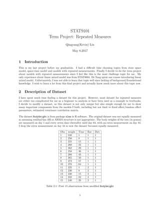
  • 1. STAT9101 Term Project: Repeated Measures Qingyang(Kevin) Liu May 8,2017 1 Introduction This is my last project before my graduation. I had a difficult time choosing topics from state space model, space-time model and models with repeated measurements. Finally I decide to do the term project about models with repeated measurements since I feel like this is the most challenge topic for me. My only experience about linear mixed model was from STAT8004. Dr.Tang spent one course introducing linear mixed model. Unfortunately, I was not able to learn that topic well since lacking of background/foundational knowledge. I wish to learn a lot from this final project and actually know much more about this topic now. 2 Description of Dataset I have spent much time finding a dataset for this project. However, most dataset for repeated measures are either too complicated for me as a beginner to analysis or have been used as a example in textbooks. I decide to modify a dataset, so this dataset is not only unique but also simple enough for me to show many important components from the models I built, including but not limit to fixed effect/random effect parameters, estimated covariance correlation matrix. The dataset BodyWeight is from package nlme in R software. The original dataset was not equally measured so assuming residual has AR or ARMA structure is not appropriate. The body weights of the rats (in grams) are measured on day 1 and every seven days thereafter until day 64, with an extra measurement on day 44. I drop the extra measurement on day 44 so now the dataset becomes equally measured. Obs weight Time Rat Diet 1 240 1 1 1 2 250 8 1 1 3 255 15 1 1 4 260 22 1 1 5 262 29 1 1 6 258 36 1 1 7 266 43 1 1 8 265 50 1 1 9 272 57 1 1 10 278 64 1 1 11 225 1 2 1 12 230 8 2 1 13 230 15 2 1 14 232 22 2 1 15 240 29 2 1 Table 2.1: First 15 observations from modified BodyWeight 1
  • 2. Table 2.1 describes the first 15 observations from modified BodyWeight. weight: body weights of rats in grams Time: days since the experiment began Rat: index for rats. Range: 1 − 16 Diet: 3 types of diets. Time (Weeks) WeightinGrams 240250260270 1 2 3 4 5 6 7 8 9 10 Rat:1 Diet:1 225230235240245 Rat:2 Diet:1 245250255260265270 1 2 3 4 5 6 7 8 9 10 Rat:3 Diet:1 255260265270275 Rat:4 Diet:1 255260265270275280 Rat:5 Diet:1 260265270275280285 Rat:6 Diet:1 260265270275280285 Rat:7 Diet:1 250260270 Rat:8 Diet:1 420440460480500 Rat:10 Diet:2 445450455460465470 Rat:11 Diet:2 560580600620 Rat:12 Diet:2 420440460480 Rat:9 Diet:2 470490510 Rat:13 Diet:3 1 2 3 4 5 6 7 8 9 10 530540550560 Rat:14 Diet:3 520530540550 Rat:15 Diet:3 1 2 3 4 5 6 7 8 9 10 510530550570 Rat:16 Diet:3 Figure 2.1: Bodyweights of all 16 rats from first week to tenth week by 3 different diets From Figure 2.1, we can get the conclusion that the increment of bodyweights varies by each rat, diet type. It is interesting to find out which factor plays a more important roles in bodyweight gain and that whether there is a difference between the effects from those three diet types. 2
  • 3. 3 Model Building For analysis of repeated measures data, there are usually three different approaches, Linear Mixed Model, MANOVA and Fixed Effect Model. In this project, I will discuss Fixed Effect Model and Linear Mixed Model. 3.1 Fixed effect model with uncorrelated residuals The first model I build only contains fixed effect Xβ. The residuals are identical independent normal dis- tributed as Var(ϵ) = σ2 I and E(ϵ) = 0. For this particular dataset, the model is Yijk = µ + αi + γk + (αγ)ik + eijk where µ: interception. αi: effect of i diet. γk: time effect at k. (αγ)ik: diet × time interaction. Yijk: weight in grams of rat j under idiet at time k. eijk: residual of rat j under i diet at time k. Cov(eijk, ei′ j′ k′ ) = 0. Time (Weeks) Residual −10−50 1 2 3 4 5 6 7 8 9 10 Rat:1 Diet:1 −30−28−26 Rat:2 Diet:1 −6−4−20 1 2 3 4 5 6 7 8 9 10 Rat:3 Diet:1 02468 Rat:4 Diet:1 2468 Rat:5 Diet:1 810121416 Rat:6 Diet:1 510152025 Rat:7 Diet:1 −6−20246 Rat:8 Diet:1 −45−35−25 Rat:10 Diet:2 −40−20 Rat:11 Diet:2 100105110 Rat:12 Diet:2 −46−44−42 Rat:9 Diet:2 −40−35−30−25 Rat:13 Diet:3 1 2 3 4 5 6 7 8 9 10 510152025 Rat:14 Diet:3 05101520 Rat:15 Diet:3 1 2 3 4 5 6 7 8 9 10 051015 Rat:16 Diet:3 Figure 3.1: Residuals from fixed effects model From Figure 3.1, we can see how implausible it is to assume Cov(eijk, ei′ j′ k′ ) = 0 since residuals that follow MVN(0, I) should fluctuate around 0 at y-axis . Next, we improve our model by assuming correlated resid- uals. 3
  • 4. Code in SAS: PROC MIXED DATA = stat9101.Termproject; CLASS Time Rat Diet; MODEL weight = diet time diet*time/S RESIDUAL OUTP = out1; RUN; 3.2 Fixed effect model with correlated residuals The fixed effect with correlated model is Yijk = µ + αi + γk + (αγ)ik + eijk where µ: interception. αi: effect of i diet. γk: time effect at k. (αγ)ik: diet × time interaction. Yijk: weight in grams of rat j under idiet at time k. eijk: residual of rat j under i diet at time k. Cov(eijk, ei′ j′ l) = 0 if either i ̸= i ′ or j ̸= j ′ . This means that within same subject, rat,correlations between measurements based on different time lag only dependent on the length of time interval. In this dataset, each rat will stick with same diet type. Hence, we only need to assume Var(eijk) = σ2 k and Cov(eijk, eijk′ ) = σkk′ We can express the vector of observations on rat j feed by diet i as Y ij = (Yij1, ..., Yjit) ′ and variance- covariance matrix of Y as Var(Y ij) = Σ, where the element in row k and column k ′ is σkk′ . Re-express variance-covariance matrix of Y as Var(Y ) = I ⊗ Σ. For this dataset, each rat is considered to have co- variance matrix Σ. In SAS Mixed procedure, the form of Σ can be specified through REPEATED statement. There are totally 17 types of covariance structures we can choose from REPEATED statement. I will build models only using some common covariance structures like compounds symmetry, unstructured, AR(1),Heterogeneous AR(1), Toeplitz,Heterogeneous Toeplitz and ARMA(1,1). Code in SAS: PROC MIXED DATA = stat9101.Termproject; CLASS time rat diet; MODEL weight = diet time diet*time/S RESIDUAL OUTP = out1; RUN; 3.2.1 Fixed effect model with unstructured covariance matrix We use ML to estimate parameters. Note that REML is the default algorithm by SAS Mixed Procedur. However, later on we need to do log-likelihood ratio test for model selection, so we choose ML instead of REML. ˆΣ =                 1159.96 1112.89 1045.90 1105.43 1104.34 1103.44 1065.59 1106.88 1033.75 1038.75 1112.89 1091.80 1034.77 1095.55 1099.77 1098.98 1066.02 1107.11 1039.22 1039.61 1045.90 1034.77 1000.98 1053.79 1059.96 1057.73 1029.73 1069.14 1006.56 1011.25 1105.43 1095.55 1053.79 1130.60 1127.87 1128.98 1100.16 1146.02 1082.13 1078.72 1104.34 1099.77 1059.96 1127.87 1139.09 1143.81 1118.96 1161.00 1101.75 1103.50 1103.44 1098.98 1057.73 1128.98 1143.81 1158.47 1134.30 1177.69 1118.22 1123.77 1065.59 1066.02 1029.73 1100.16 1118.96 1134.30 1121.10 1160.33 1108.88 1114.88 1106.88 1107.11 1069.14 1146.02 1161.00 1177.69 1160.33 1211.34 1151.59 1162.52 1033.75 1039.22 1006.56 1082.13 1101.75 1118.22 1108.88 1151.59 1107.19 1117.91 1038.75 1039.61 1011.25 1078.72 1103.50 1123.77 1114.88 1162.52 1117.91 1153.33                 4
  • 5. Note that covariance matrix is symmetric. ˆΣ = ˆΣ t The unstructured covariance is the most complicated structure, which contains 11 × 10/2 = 55 parame- ters. The variances on the diagonal of this covariance matrix are the estimated variances of measures from week1 to week 10. The covariance σi,k measures the covariance between week i and week k. For example, σ1,2 = 1112.89 is covariance between measures week 1 and week 2. The correlation matrix of residual, which equals to corr(ϵ) = (diag(Σ)) − 1 2 Σ (diag(Σ)) − 1 2 , is shown below. corr(ϵ) =                 1.000 0.989 0.971 0.965 0.961 0.952 0.934 0.934 0.912 0.898 0.989 1.000 0.990 0.986 0.986 0.977 0.964 0.963 0.945 0.927 0.971 0.990 1.000 0.991 0.993 0.982 0.972 0.971 0.956 0.941 0.965 0.986 0.991 1.000 0.994 0.987 0.977 0.979 0.967 0.945 0.961 0.986 0.993 0.994 1.000 0.996 0.990 0.988 0.981 0.963 0.952 0.977 0.982 0.987 0.996 1.000 0.995 0.994 0.987 0.972 0.934 0.964 0.972 0.977 0.990 0.995 1.000 0.996 0.995 0.981 0.934 0.963 0.971 0.979 0.988 0.994 0.996 1.000 0.994 0.984 0.912 0.945 0.956 0.967 0.981 0.987 0.995 0.994 1.000 0.989 0.898 0.927 0.941 0.945 0.963 0.972 0.981 0.984 0.989 1.000                 For example the correlation for residual of weight measures between week1 and week2, can be found in the first row, second column of the correlation matrix above. We can see that the longer of the time lags spans, the smaller correlation is. In other words, residuals of weight measurement at week1 has weaker influence on residuals of weight measurement at week3 or on following weeks than residuals of weight measurement at week2. This makes logical sense. We can use this property of decaying correlation to do model comparison. We will also do model comparison by using information criterion and log-likelihood test. The information criterion could be found in table 3.1 Fit Statistics -2 Log Likelihood 879 AIC (Smaller is Better) 1049 AICC (Smaller is Better) 1246.6 BIC (Smaller is Better) 1114.7 Table 3.1: Information criterion of fixed effect model with unstructured covariance matrix Null Model Likelihood Ratio Test DF Chi-Square Pr >ChiSq 54 699.47 <.0001 Table 3.2: Null Model Likelihood Ratio Test with unstructured covariance matrix Table 3.2 shows the results of null model likelihood ratio test. The null hypothesis is that the null model, which is fixed effect model with uncorrelated residual,Σ = σ2 I, fits as good as the model with the specified covariance structure. The alternative hypothesis is that the model with more parameters fit better than the null model does. The degree of freedom,54 = 55 − 1, is determined by the difference between the number of parameters of null model and model with more parameters. Since the p-value is smaller than 0.0001, we confirm the conclusion we get in section 3.1, fixed effect model with uncorrelated residuals is inadequate. 5
  • 6. Type 3 Tests of Fixed Effects Effect Num DF Den DF F Value Pr >F Diet 2 13 107.78 <.0001 Time 9 13 66.16 <.0001 Time*Diet 18 13 19.76 <.0001 Table 3.3: Tests of Fixed Effects with unstructured covariance matrix From the result of table 3.3, we have that under fixed effects model with unstructured covariance, all three fixed effect, diet, time and interaction between diet and time have significant effect on rats’ bodyweight. We still need to try other models with different covariance structure and recheck our conclusion here. Code in SAS: PROC MIXED DATA = stat9101.Termproject METHOD = ML; CLASS time rat diet; MODEL weight = diet time diet*time/S RESIDUAL OUTP = out2; REPEATED time / SUBJECT = rat(diet) TYPE = UN R RCORR; RUN; 3.2.2 Fixed effect model with compound symmetry covariance matrix: a inadequate model The compound symmetry structure: Σ =        σ2 + σ1 σ1 σ1 . . . σ1 σ2 + σ1 σ1 . . . σ1 ... ... ... σ2 + σ1 σ1 σ2 + σ1        There are two parameters, σ and σ1 for the compound symmetry structure. Covariance Parameter Estimates Cov Parm Subject Estimate CS Rat(Diet) 1094.42 Residual 32.9609 Table 3.4: Covariance Parameter Estimates for compound symmetry structure From table 3.4 we have σ1 = 1094.42 and σ2 = 32.9609. We have estimated covariance matrix of residuals like following: ˆΣ =                 1127.39 1094.42 1094.42 1094.42 1094.42 1094.42 1094.42 1094.42 1094.42 1094.42 1094.42 1127.39 1094.42 1094.42 1094.42 1094.42 1094.42 1094.42 1094.42 1094.42 1094.42 1094.42 1127.39 1094.42 1094.42 1094.42 1094.42 1094.42 1094.42 1094.42 1094.42 1094.42 1094.42 1127.39 1094.42 1094.42 1094.42 1094.42 1094.42 1094.42 1094.42 1094.42 1094.42 1094.42 1127.39 1094.42 1094.42 1094.42 1094.42 1094.42 1094.42 1094.42 1094.42 1094.42 1094.42 1127.39 1094.42 1094.42 1094.42 1094.42 1094.42 1094.42 1094.42 1094.42 1094.42 1094.42 1127.39 1094.42 1094.42 1094.42 1094.42 1094.42 1094.42 1094.42 1094.42 1094.42 1094.42 1127.39 1094.42 1094.42 1094.42 1094.42 1094.42 1094.42 1094.42 1094.42 1094.42 1094.42 1127.39 1094.42 1094.42 1094.42 1094.42 1094.42 1094.42 1094.42 1094.42 1094.42 1094.42 1127.39                 6
  • 7. We can hand check the first number in estimated covariance matrix: 1127.39 ≈ 1094.42 + 32.9609 Correlation matrix as: corr(ϵ) =                 1.0000 0.9708 0.9708 0.9708 0.9708 0.9708 0.9708 0.9708 0.9708 0.9708 0.9708 1.0000 0.9708 0.9708 0.9708 0.9708 0.9708 0.9708 0.9708 0.9708 0.9708 0.9708 1.0000 0.9708 0.9708 0.9708 0.9708 0.9708 0.9708 0.9708 0.9708 0.9708 0.9708 1.0000 0.9708 0.9708 0.9708 0.9708 0.9708 0.9708 0.9708 0.9708 0.9708 0.9708 1.0000 0.9708 0.9708 0.9708 0.9708 0.9708 0.9708 0.9708 0.9708 0.9708 0.9708 1.0000 0.9708 0.9708 0.9708 0.9708 0.9708 0.9708 0.9708 0.9708 0.9708 0.9708 1.0000 0.9708 0.9708 0.9708 0.9708 0.9708 0.9708 0.9708 0.9708 0.9708 0.9708 1.0000 0.9708 0.9708 0.9708 0.9708 0.9708 0.9708 0.9708 0.9708 0.9708 0.9708 1.0000 0.9708 0.9708 0.9708 0.9708 0.9708 0.9708 0.9708 0.9708 0.9708 0.9708 1.0000                 where 0.9708 = 1094.42/1127.39 From estimated correlation matrix, we can see that compound symmetry structure may be inappropriate for this dataset. Because the correlation of weight measures between different time lags does not vary. We confirm this guess using following methods. Fit Statistics -2 Log Likelihood 1106.2 AIC (Smaller is Better) 1170.2 AICC (Smaller is Better) 1186.9 BIC (Smaller is Better) 1195.0 Table 3.5: Information Criterion for fixed effects model with compound symmetry structure By comparing table 3.5 and table 3.1, we find fixed effects model with compound symmetry structure has larger information criterion. By using log-likelihood test, we have p-value < 0.001 where χ2 = 1106.2−879 = 227.2, df = 55 − 2. Based on the result of comparing information criterion and log-likelihood test, we get the conclusion that model with unstructured covariance are is more adequate than model with compound symmetry structure. Type 3 Tests of Fixed Effects Effect Num DF Den DF F Value Pr >F Diet 2 13 107.78 <.0001 Time 9 117 90.19 <.0001 Time*Diet 18 117 8.27 <.0001 Table 3.6: Type 3 Tests of Fixed Effects with compound symmetry structure According to table 3.6, our conclusion from section 3.2.1 remains the same, that all three fixed effect, diet, time and interaction between diet and time have significant effect on rats’ bodyweight. Code in R > pchisq(227.2,df = 55-2, lower.tail = F) [1] 1.946558e-23 7
  • 8. Code in SAS PROC MIXED DATA = stat9101.Termproject METHOD = ML; CLASS time rat diet; MODEL weight = diet time diet*time/S RESIDUAL OUTP = out2; REPEATED time / SUBJECT = rat(diet) TYPE = CS R RCORR; RUN; 3.2.3 Fixed effect model with AR(1) structure and other common structures The AR(1) structure: Σ = σ2     1.0 ρ ρ2 ρ3 1.0 ρ ρ2 1.0 ρ 1.0     There are two parameters of this covariance structure. Covariance Parameter Estimates Cov Parm Subject Estimate AR(1) Rat(Diet) 0.9923 Residual 1154.53 Table 3.7: Covariance Parameter Estimates for AR(1) structure From table 3.7, we have σ2 = 1154.53, ρ = 0.9923 and the estimated covariance matrix as ˆΣ =                 1154.53 1145.65 1136.83 1128.08 1119.40 1110.79 1102.24 1093.75 1085.34 1076.98 1145.65 1154.53 1145.65 1136.83 1128.08 1119.40 1110.79 1102.24 1093.75 1085.34 1136.83 1145.65 1154.53 1145.65 1136.83 1128.08 1119.40 1110.79 1102.24 1093.75 1128.08 1136.83 1145.65 1154.53 1145.65 1136.83 1128.08 1119.40 1110.79 1102.24 1119.40 1128.08 1136.83 1145.65 1154.53 1145.65 1136.83 1128.08 1119.40 1110.79 1110.79 1119.40 1128.08 1136.83 1145.65 1154.53 1145.65 1136.83 1128.08 1119.40 1102.24 1110.79 1119.40 1128.08 1136.83 1145.65 1154.53 1145.65 1136.83 1128.08 1093.75 1102.24 1110.79 1119.40 1128.08 1136.83 1145.65 1154.53 1145.65 1136.83 1085.34 1093.75 1102.24 1110.79 1119.40 1128.08 1136.83 1145.65 1154.53 1145.65 1076.98 1085.34 1093.75 1102.24 1110.79 1119.40 1128.08 1136.83 1145.65 1154.53                 Estimated correlation matrix as corr(ϵ) =                 1.000 0.992 0.985 0.977 0.970 0.962 0.955 0.947 0.940 0.933 0.992 1.000 0.992 0.985 0.977 0.970 0.962 0.955 0.947 0.940 0.985 0.992 1.000 0.992 0.985 0.977 0.970 0.962 0.955 0.947 0.977 0.985 0.992 1.000 0.992 0.985 0.977 0.970 0.962 0.955 0.970 0.977 0.985 0.992 1.000 0.992 0.985 0.977 0.970 0.962 0.962 0.970 0.977 0.985 0.992 1.000 0.992 0.985 0.977 0.970 0.955 0.962 0.970 0.977 0.985 0.992 1.000 0.992 0.985 0.977 0.947 0.955 0.962 0.970 0.977 0.985 0.992 1.000 0.992 0.985 0.940 0.947 0.955 0.962 0.970 0.977 0.985 0.992 1.000 0.992 0.933 0.940 0.947 0.955 0.962 0.970 0.977 0.985 0.992 1.000                 Now the correlation between different time lags begins to decays. It would be very tedious to show the estimated covariance and correlation matrix of all 7 models. I will use information criterion as a model selection tool to choose the best model. 8
  • 9. Fit Statistics-AR(1) Fit Statistics-ARH(1) Fit Statistics-ARMA(1,1) -2 Log Likelihood 980.7 -2 Log Likelihood 970 -2 Log Likelihood 979.5 AIC (Smaller is Better) 1044.7 AIC (Smaller is Better) 1052 AIC (Smaller is Better) 1045.5 AICC (Smaller is Better) 1061.3 AICC (Smaller is Better) 1081.2 AICC (Smaller is Better) 1063.3 BIC (Smaller is Better) 1069.4 BIC (Smaller is Better) 1083.7 BIC (Smaller is Better) 1071.0 Fit Statistics-Unstructured Fit Statistics-Toeplitz Fit Statistics-Heterogeneous Toeplitz -2 Log Likelihood 879.0 -2 Log Likelihood 967.0 -2 Log Likelihood 954.3 AIC (Smaller is Better) 1049.0 AIC (Smaller is Better) 1047.0 AIC (Smaller is Better) 1052.3 AICC (Smaller is Better) 1246.6 AICC (Smaller is Better) 1074.5 AICC (Smaller is Better) 1096.8 BIC (Smaller is Better) 1114.7 BIC (Smaller is Better) 1077.9 BIC (Smaller is Better) 1090.1 Table 3.8: Information Criterion Note that the information criterion for compound symmetry is not in table 3.8 but in table 3.5. Overall fixed effect model with AR(1) structure is indeed the best model between these 7 models. Type 3 Tests of Fixed Effects Effect Num DF Den DF F Value Pr >F Diet 2 13 105.10 <.0001 Time 9 117 27.71 <.0001 Time*Diet 18 117 5.69 <.0001 Table 3.9: Test of Fixed Effects - AR(1) structure From table 3.9, we have the conclusion that all three fixed effect, diet, time and interaction between diet and time have significant effect on rats’ bodyweight. From table 3.10, the difference between effects from diet1 and diet3 are significant all the time, so is the difference between effect from diet1 and diet2.The difference between diet2 and diet3 is significant until time lag 8(week2).Table 3.10 was created through SAS PROC GLIMMIX. The results from SAS PROC GLIMMIX and SAS PROC MIXED is negligible. From table 3.11, we have that the bodyweight of rats by diet1 increases faster than other diet types since the estimated parameters for interaction between time and diet1 are positive and significantly different from zero all the time. The intercept of fixed effect from diet2 is not significant since p-value is 0.21. The time effects are significant from first week to last week. All rats will gain weights while time lag increases. The interaction between time and diet2 becomes insignificant after time lag8(week2). This finding is as same as what we have from table 3.10. Code in SAS: proc mixed data = stat9101.Termproject; class Time Rat Diet; model weight = diet time diet*time/S; repeated time/ subject = rat type = AR(1) R; run; proc glimmix data = stat9101.Termproject outdesign = design1; class Time Rat Diet; model weight = diet time diet*time; random time/ subject = rat residual type = AR(1) S G; run; proc mixed data = stat9101.Termproject; class Time Rat Diet; 9
  • 10. model weight = diet time diet*time/S; repeated time/ subject = rat type = AR(1) R; random Rat/G S; run; proc glimmix data = stat9101.Termproject outdesign = design2; class Time Rat Diet; model weight = diet time diet*time/S; random time/ subject = rat residual type = AR(1); random Rat/G S; run; /*Fixed Model*/ PROC MIXED DATA = stat9101.Termproject; CLASS time rat diet; MODEL weight = diet time diet*time/S RESIDUAL OUTP = out1; RUN; /*Fixed Model with unstrcucred matrix*/ PROC MIXED DATA = stat9101.Termproject METHOD = ML; CLASS time rat diet; MODEL weight = diet time diet*time/S RESIDUAL OUTP = out2; REPEATED time / SUBJECT = rat(diet) TYPE = UN R RCORR; RUN; /*Fixed Model with compound symmetry matrix*/ PROC MIXED DATA = stat9101.Termproject METHOD = ML; CLASS time rat diet; MODEL weight = diet time diet*time/S RESIDUAL OUTP = out2; REPEATED time / SUBJECT = rat(diet) TYPE = CS R RCORR; RUN; /*Fixed Model with AR(1)*/ PROC MIXED DATA = stat9101.Termproject METHOD = ML; CLASS time rat diet; MODEL weight = diet time diet*time/S RESIDUAL OUTP = out1; REPEATED time / SUBJECT = rat(diet) TYPE = AR(1) R RCORR; RUN; /*Fixed Model with ARH(1)*/ PROC MIXED DATA = stat9101.Termproject METHOD = ML; CLASS time rat diet; MODEL weight = diet time diet*time/S RESIDUAL OUTP = out1; REPEATED time / SUBJECT = rat(diet) TYPE = ARH(1) R RCORR; RUN; /*Fixed Model with Toeplitz*/ PROC MIXED DATA = stat9101.Termproject METHOD = ML; CLASS time rat diet; MODEL weight = diet time diet*time/S RESIDUAL OUTP = out1; REPEATED time / SUBJECT = rat(diet) TYPE = TOEP R RCORR; RUN; /*Fixed Model with Heterogeneous Toeplitz*/ PROC MIXED DATA = stat9101.Termproject METHOD = ML; CLASS time rat diet; MODEL weight = diet time diet*time/S RESIDUAL OUTP = out1; REPEATED time / SUBJECT = rat(diet) TYPE = TOEPH R RCORR; RUN; /*Fixed Model with ARMA(1,1)*/ PROC MIXED DATA = stat9101.Termproject METHOD = ML; CLASS time rat diet; 10
  • 11. MODEL weight = diet time diet*time/S RESIDUAL OUTP = out1; REPEATED time / SUBJECT = rat(diet) TYPE = ARMA(1,1) R RCORR; RUN; /*SIMPLE EFFECT COMPARISON*/ PROC GLIMMIX DATA = stat9101.Termproject NOREML OUTDESIGN = OUT1; CLASS time(REF = FIRST) rat diet(REF = FIRST); MODEL weight = diet time diet*time/S; RANDOM _RESIDUAL_/ TYPE = AR(1) SUBJECT = rat(diet); RUN; Simple Effect Comparisons of Time*Diet Least Squares Means By Time Simple Effect Level Diet _Diet Estimate Standard Error DF t Value Pr >|t| Time 1 1 2 -203.13 20.81 117.00 -9.76 <.0001 Time 1 1 3 -258.13 20.81 117.00 -12.41 <.0001 Time 1 2 3 -55.00 24.03 117.00 -2.29 0.0200 Time 8 1 2 -205.00 20.81 117.00 -9.85 <.0001 Time 8 1 3 -251.25 20.81 117.00 -12.08 <.0001 Time 8 2 3 -46.25 24.03 117.00 -1.92 0.0600 Time 15 1 2 -213.13 20.81 117.00 -10.24 <.0001 Time 15 1 3 -259.38 20.81 117.00 -12.47 <.0001 Time 15 2 3 -46.25 24.03 117.00 -1.92 0.0600 Time 22 1 2 -213.13 20.81 117.00 -10.24 <.0001 Time 22 1 3 -256.38 20.81 117.00 -12.32 <.0001 Time 22 2 3 -43.25 24.03 117.00 -1.80 0.0700 Time 29 1 2 -218.13 20.81 117.00 -10.48 <.0001 Time 29 1 3 -259.13 20.81 117.00 -12.45 <.0001 Time 29 2 3 -41.00 24.03 117.00 -1.71 0.0900 Time 36 1 2 -223.75 20.81 117.00 -10.75 <.0001 Time 36 1 3 -264.25 20.81 117.00 -12.70 <.0001 Time 36 2 3 -40.50 24.03 117.00 -1.69 0.0900 Time 43 1 2 -219.12 20.81 117.00 -10.53 <.0001 Time 43 1 3 -255.37 20.81 117.00 -12.27 <.0001 Time 43 2 3 -36.25 24.03 117.00 -1.51 0.1300 Time 50 1 2 -231.75 20.81 117.00 -11.14 <.0001 Time 50 1 3 -268.75 20.81 117.00 -12.92 <.0001 Time 50 2 3 -37.00 24.03 117.00 -1.54 0.1300 Time 57 1 2 -237.50 20.81 117.00 -11.41 <.0001 Time 57 1 3 -271.00 20.81 117.00 -13.02 <.0001 Time 57 2 3 -33.50 24.03 117.00 -1.39 0.1700 Time 64 1 2 -244.75 20.81 117.00 -11.76 <.0001 Time 64 1 3 -276.50 20.81 117.00 -13.29 <.0001 Time 64 2 3 -31.75 24.03 117.00 -1.32 0.1900 Table 3.10: Simple Effect Comparisons of Time*Diet Least Squares Means By Time by PROC GLIMMIX 11
  • 12. Solution for Fixed Effects Effect Time Diet Estimate Standard Error DF t Value Pr >|t| Intercept 550.25 16.99 13.00 32.39 <.0001 Diet 1 -276.50 20.81 13.00 -13.29 <.0001 Diet 2 -31.75 24.03 13.00 -1.32 0.21 Diet 3 0.00 . . . . Time 1 -41.50 6.23 117.00 -6.66 <.0001 Time 8 -44.00 5.88 117.00 -7.48 <.0001 Time 15 -36.50 5.51 117.00 -6.62 <.0001 Time 22 -32.00 5.11 117.00 -6.26 <.0001 Time 29 -26.50 4.68 117.00 -5.67 <.0001 Time 36 -21.00 4.19 117.00 -5.01 <.0001 Time 43 -27.50 3.64 117.00 -7.56 <.0001 Time 50 -12.00 2.98 117.00 -4.03 <.0001 Time 57 -7.75 2.11 117.00 -3.68 0.00 Time 64 0.00 . . . . Time*Diet 1 1 18.38 7.63 117.00 2.41 0.02 Time*Diet 1 2 -23.25 8.81 117.00 -2.64 0.01 Time*Diet 1 3 0.00 . . . . Time*Diet 8 1 25.25 7.20 117.00 3.51 0.00 Time*Diet 8 2 -14.50 8.32 117.00 -1.74 0.08 Time*Diet 8 3 0.00 . . . . Time*Diet 15 1 17.13 6.75 117.00 2.54 0.01 Time*Diet 15 2 -14.50 7.80 117.00 -1.86 0.07 Time*Diet 15 3 0.00 . . . . Time*Diet 22 1 20.13 6.26 117.00 3.21 0.00 Time*Diet 22 2 -11.50 7.23 117.00 -1.59 0.11 Time*Diet 22 3 0.00 . . . . Time*Diet 29 1 17.38 5.73 117.00 3.03 0.00 Time*Diet 29 2 -9.25 6.61 117.00 -1.40 0.16 Time*Diet 29 3 0.00 . . . . Time*Diet 36 1 12.25 5.13 117.00 2.39 0.02 Time*Diet 36 2 -8.75 5.93 117.00 -1.48 0.14 Time*Diet 36 3 0.00 . . . . Time*Diet 43 1 21.13 4.45 117.00 4.74 <.0001 Time*Diet 43 2 -4.50 5.14 117.00 -0.87 0.38 Time*Diet 43 3 0.00 . . . . Time*Diet 50 1 7.75 3.64 117.00 2.13 0.04 Time*Diet 50 2 -5.25 4.21 117.00 -1.25 0.21 Time*Diet 50 3 0.00 . . . . Time*Diet 57 1 5.50 2.58 117.00 2.13 0.04 Time*Diet 57 2 -1.75 2.98 117.00 -0.59 0.56 Time*Diet 57 3 0.00 . . . . Time*Diet 64 1 0.00 . . . . Time*Diet 64 2 0.00 . . . . Time*Diet 64 3 0.00 . . . . Table 3.11: Fixed Effect analysis-AR(1) 12
  • 13. 3.3 Linear Mixed Model-with fixed and random effect - inappropriate model It is very nature to consider the subject of this experiment, rats, as random effect. Now we will have another covariance matrix G. The linear mixed model is: y = Xβ + Zγ + ϵ where ( γ ϵ ) ∼ N (( 0 0 ) ( G 0 0 R )) Assuming ϵ has AR(1) structure, we get ˆG matrix and ˆR matrix below by MIVQUE0 method instead of REML or MLE. SAS software can’t estimate G matrix by REML or ML method. The SAS console shows Estimated G matrix is not positive definite. I don’t know much about the difference between MIVQUE0 and MLE or REMLE(I do know the difference between MLE and REMLE). According to SAS MIXED PROCEDURE MANUAL 14.1, MIVQUE0 method is a non-iterative method and in fact estimates starting values for the ML and REMLE methods. MIVQUE0 method turns out to be the only method that esitmates ˆR matrix successfully. ˆR =                 46.975 32.040 21.853 14.905 10.166 6.934 4.729 3.226 2.200 1.501 32.040 46.975 32.040 21.853 14.905 10.166 6.934 4.729 3.226 2.200 21.853 32.040 46.975 32.040 21.853 14.905 10.166 6.934 4.729 3.226 14.905 21.853 32.040 46.975 32.040 21.853 14.905 10.166 6.934 4.729 10.166 14.905 21.853 32.040 46.975 32.040 21.853 14.905 10.166 6.934 6.934 10.166 14.905 21.853 32.040 46.975 32.040 21.853 14.905 10.166 4.729 6.934 10.166 14.905 21.853 32.040 46.975 32.040 21.853 14.905 3.226 4.729 6.934 10.166 14.905 21.853 32.040 46.975 32.040 21.853 2.200 3.226 4.729 6.934 10.166 14.905 21.853 32.040 46.975 32.040 1.501 2.200 3.226 4.729 6.934 10.166 14.905 21.853 32.040 46.975                 Estimated G Matrix Row Effect Rat Diet Col1 Col2 Col3 Col4 Col5 Col6 Col7 Col8 Col9 Col10 Col11 Col12 Col13 Col14 Col15 Col16 1 Rat(Diet) 1 1 1340.58 2 Rat(Diet) 2 1 1340.58 3 Rat(Diet) 3 1 1340.58 4 Rat(Diet) 4 1 1340.58 5 Rat(Diet) 5 1 1340.58 6 Rat(Diet) 6 1 1340.58 7 Rat(Diet) 7 1 1340.58 8 Rat(Diet) 8 1 1340.58 9 Rat(Diet) 9 2 1340.58 10 Rat(Diet) 10 2 1340.58 11 Rat(Diet) 11 2 1340.58 12 Rat(Diet) 12 2 1340.58 13 Rat(Diet) 13 3 1340.58 14 Rat(Diet) 14 3 1340.58 15 Rat(Diet) 15 3 1340.58 16 Rat(Diet) 16 3 1340.58 Table 3.12: Estimated ˆG matrix The ˆG is shown in table 3.12, not in matrix form since the first four columns explains the meaning of this matrix very well. This diagonal form matrix implies that covariance between different rats is zero. It plau- sible to assume that effects on different rats are independent. From table 3.13, we have that adding random effect is not necessary for this dataset. The model with random effects have 1 more parameter for ˆG and 16 more parameters for random slopes. Adding more parameters 13
  • 14. without improving the model increases information criterion. We can not compare table 3.8 and table 3.13 since they are created by ML and MIVQUE0 methods respectively. Fit Statistics-no random effects Fit Statistics-with random effect -2 Res Log Likelihood 877.5 -2 Res Log Likelihood 891.6 AIC (Smaller is Better) 881.5 AIC (Smaller is Better) 897.6 AICC (Smaller is Better) 881.6 AICC (Smaller is Better) 897.8 BIC (Smaller is Better) 883.0 BIC (Smaller is Better) 900.0 Table 3.13: Information criterion-by MIVQUE0 method From table 3.14, we have that based on linear mixed model (even though it is not necessary to add random effect),all three fixed effect, diet, time and interaction between diet and time have significant effect on rats’ bodyweight. Type 3 Tests of Fixed Effects Effect Num DF Den DF F Value Pr >F Diet 2 13 87.04 <.0001 Time 9 117 37.96 <.0001 Time*Diet 18 117 5 <.0001 Table 3.14: Fixed effect analysis from linear mixed model Solution for Random Effects Effect Rat Diet Estimate Std Err Pred DF t Value Pr >|t| Rat(Diet) 1 1 -2.853 13.513 117.000 -0.210 0.833 Rat(Diet) 2 1 -26.269 13.513 117.000 -1.940 0.054 Rat(Diet) 3 1 -4.206 13.513 117.000 -0.310 0.756 Rat(Diet) 4 1 3.397 13.513 117.000 0.250 0.802 Rat(Diet) 5 1 5.538 13.513 117.000 0.410 0.683 Rat(Diet) 6 1 10.089 13.513 117.000 0.750 0.457 Rat(Diet) 7 1 13.170 13.513 117.000 0.970 0.332 Rat(Diet) 8 1 1.135 13.513 117.000 0.080 0.933 Rat(Diet) 9 2 -42.881 18.655 117.000 -2.300 0.023 Rat(Diet) 10 2 -33.148 18.655 117.000 -1.780 0.078 Rat(Diet) 11 2 -28.221 18.655 117.000 -1.510 0.133 Rat(Diet) 12 2 104.250 18.655 117.000 5.590 <.0001 Rat(Diet) 13 3 -32.678 18.655 117.000 -1.750 0.082 Rat(Diet) 14 3 13.148 18.655 117.000 0.700 0.482 Rat(Diet) 15 3 11.299 18.655 117.000 0.610 0.546 Rat(Diet) 16 3 8.231 18.655 117.000 0.440 0.660 Table 3.15: Solution for Random Effects 14
  • 15. Solution for Fixed Effects Effect Time Diet Estimate Standard Error DF t Value Pr >|t| Intercept 550.25 18.6249 13 29.54 <.0001 Diet 1 -276.5 22.8108 13 -12.12 <.0001 Diet 2 -31.75 26.3396 13 -1.21 0.2495 Diet 3 0 . . . . Time 1 -41.5 4.7684 117 -8.7 <.0001 Time 8 -44 4.7316 117 -9.3 <.0001 Time 15 -36.5 4.6771 117 -7.8 <.0001 Time 22 -32 4.596 117 -6.96 <.0001 Time 29 -26.5 4.4745 117 -5.92 <.0001 Time 36 -21 4.2901 117 -4.9 <.0001 Time 43 -27.5 4.0044 117 -6.87 <.0001 Time 50 -12 3.5442 117 -3.39 0.001 Time 57 -7.75 2.7327 117 -2.84 0.0054 Time 64 0 . . . . Time*Diet 1 1 18.375 5.84 117 3.15 0.0021 Time*Diet 1 2 -23.25 6.7435 117 -3.45 0.0008 Time*Diet 1 3 0 . . . . Time*Diet 8 1 25.25 5.7949 117 4.36 <.0001 Time*Diet 8 2 -14.5 6.6914 117 -2.17 0.0323 Time*Diet 8 3 0 . . . . Time*Diet 15 1 17.125 5.7282 117 2.99 0.0034 Time*Diet 15 2 -14.5 6.6143 117 -2.19 0.0303 Time*Diet 15 3 0 . . . . Time*Diet 22 1 20.125 5.6289 117 3.58 0.0005 Time*Diet 22 2 -11.5 6.4997 117 -1.77 0.0794 Time*Diet 22 3 0 . . . . Time*Diet 29 1 17.375 5.4801 117 3.17 0.0019 Time*Diet 29 2 -9.25 6.3278 117 -1.46 0.1465 Time*Diet 29 3 0 . . . . Time*Diet 36 1 12.25 5.2542 117 2.33 0.0214 Time*Diet 36 2 -8.75 6.0671 117 -1.44 0.1519 Time*Diet 36 3 0 . . . . Time*Diet 43 1 21.125 4.9044 117 4.31 <.0001 Time*Diet 43 2 -4.5 5.6631 117 -0.79 0.4284 Time*Diet 43 3 0 . . . . Time*Diet 50 1 7.75 4.3407 117 1.79 0.0768 Time*Diet 50 2 -5.25 5.0122 117 -1.05 0.2971 Time*Diet 50 3 0 . . . . Time*Diet 57 1 5.5 3.3469 117 1.64 0.103 Time*Diet 57 2 -1.75 3.8647 117 -0.45 0.6515 Time*Diet 57 3 0 . . . . Time*Diet 64 1 0 . . . . Time*Diet 64 2 0 . . . . Time*Diet 64 3 0 . . . . Table 3.16: Solution for Fixed Effects 15
  • 16. The estimated ˆβ and ˆγ could be found in table 3.16 and table 3.15 respectively. It is easy to find out that many estimated parameters in table 3.15 are not significantly different from 0, this confirms the conclusion that adding random effect is not nessccary for this dataset. Code in SAS: /*RANDOM EFFECT MODEL*/ PROC MIXED DATA = stat9101.Termproject METHOD = MIVQUE0; CLASS time rat diet; MODEL weight = diet time diet*time/S RESIDUAL OUTP = out1; REPEATED time / SUBJECT = rat(diet) TYPE = AR(1) R RCORR; RANDOM rat(diet)/S G; RUN; /*FIXED EEFECT MODEL*/ PROC MIXED DATA = stat9101.Termproject METHOD = MIVQUE0; CLASS time rat diet; MODEL weight = diet time diet*time/S RESIDUAL OUTP = out1; REPEATED time / SUBJECT = rat(diet) TYPE = AR(1) R RCORR; RUN; 16
  • 17. 4 Influence Analysis of Fixed effect model with AR(1) structure 1 2 3 4 5 6 7 8 9 10 11 12 13 14 15 16 Deleted Rat 0 2 4 6 8 10 Distance Likelihood Distance Influence Statistics for Fixed Effects 1 2 3 4 5 6 7 8 9 10 11 12 13 14 15 16 Deleted Rat 0 10 20 30 40 COVRATIO 1 2 3 4 5 6 7 8 9 10 11 12 13 14 15 16 0.00 0.05 0.10 0.15 0.20 0.25 Cook'sD Figure 4.1: Influence analysis figures The main purpose of analysis of repeated measures data is usually to study the influence of cluster(rats) by checking ANOVA table of fixed effect like table 3.14, rather than the influence of individual observa- tions. However, sometimes unfitted observations or outliers show us some important informations we did not expect. Figure 4.1 contains three sub-figures, likelihood distance, Cook’s Distance and COVRATIO. Likelihood distance and Cook’ distance acutally have exactly same trend. This shows us that fixed effect model with AR(1) structure does not fit rat 12(diet2), 15(diet3) and 16(diet3) very well. COVRATIO shows us that rat 9(diet2) has the most significant influence on covariance estimation. It is important to inform other scientists to check those rats. Other scientists may find important facts hide in those data. Table 4.1 contains the data for figure 4.1. The column, number of observations in level, means that each rat has been measured 10 times. 17
  • 18. Influence Diagnostics for Levels of Rat Rat Number of Observations in Level Cook’s D COVRATIO Likelihood Distance 1 10 0.05208 3.149 1.575 2 10 0.05759 2.493 1.768 3 10 0.01964 12.037 0.684 4 10 0.03734 5.835 1.121 5 10 0.02827 8.475 0.882 6 10 0.03527 6.357 1.063 7 10 0.08014 0.939 2.695 8 10 0.04198 4.813 1.254 9 10 0.06899 37.546 2.068 10 10 0.13364 11.805 4.079 11 10 0.16226 6.971 5.100 12 10 0.21294 2.679 7.129 13 10 0.13539 11.434 4.139 14 10 0.18676 4.408 6.044 15 10 0.27533 0.790 10.054 16 10 0.23598 1.717 8.151 Table 4.1: Influence diagnostics for each rat Code in SAS: /*INFLUENCE ANALYSIS*/ PROC MIXED DATA = stat9101.Termproject METHOD = ML; CLASS time rat diet; MODEL weight = diet time diet*time/S RESIDUAL OUTP = out1 INFLUENCE(EFFECT = rat); REPEATED time / SUBJECT = rat(diet) TYPE = AR(1) R RCORR; ODS SELECT influence; RUN; 5 Conclusion Based on all models we used in this paper, we have a solid conclusion that time, diet types and interaction between time and diet types have significant influence on rats’ weight. Diet1 is the most effective diet for rats to gain weight. The detailed comparison between diet1, diet2 and diet3 can be found in section 3.2.3. Among all models we tried in this project, fixed effect model with AR(1) structure is the most appropriate one. There are some important things I need to point out that all these 16 rats have different initial body weights, we can make our conclusion more reliable by using rats that have similar initial weights and adding more informations about those rats like health status and ages. References [1] SAS/STAT 14.1 User’s Guide The MIXED Procedure [2] SAS/STAT 14.1 User’s Guide The GLIMMIX Procedure [3] Ramon C.Littell, Ph.D, SAS for Mixed Models, Second Edition [4] Alan Agresti, Ph.D, Foundations of Linear and Generalized Linear Models, First Edition [5] Charles E. McCulloch, Shayle R. Searle, Generalized, Linear, and Mixed Models 18