Streamlining Python Development: A Guide to a Modern Project Setup
Fundamentals of gps receivers
1. Chapter 2
Introduction to the Global Positioning System
In Chap. 1 we introduced some of the working principles of the GPS by analogy
with a simple linear model. Now its time to move into more detailed discussion of
the GPS satellite system and how it works. In this chapter we will cover the basics
of how the satellites are configured, making the path delay measurements, a quick
look at the user position solution equations, and a high-level block diagram of GPS
receiver will be presented.
2.1 The Satellite System
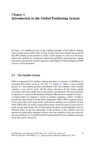
GPS is comprised of 24 satellites orbiting the earth at a distance of 20,000 km as
measured from mean sea level. See Fig. 2.1. Figure 2.2 shows a more detailed
picture of a user getting position information from four satellites. Each satellite
contains a very precise clock. All the clocks and hence all the timing signals
associated with each satellite are in near-perfect synchronism. The basic principle
of operation is similar to the Roadway Distance Measurement example of Chap. 1.
A rough model is to imagine a system of satellites emitting a “pulse” of light at
exactly the same instant as all the others (Important: GPS is NOT a pulsed system).
If you were at the exact center of the earth and the satellites were in perfect circular
orbits (GPS orbits are nearly circular) these pulses would all arrive at your receiver
at the exactly same instant. For all other points the pulses would (typically) arrive at
different times. If one has knowledge of the positions of the satellites and can
measure the path delay (distance) from at least four satellites to the user receiver,
the user position X, Y, Z in ECEF (Earth Centered Earth Fixed) coordinates and user
clock bias can be solved for.
D. Doberstein, Fundamentals of GPS Receivers: A Hardware Approach, 23
DOI 10.1007/978-1-4614-0409-5_2, # Springer Science+Business Media, LLC 2012
2. 24 2 Introduction to the Global Positioning System
c DKD INSTRUMENTS
EARTH
c DKD INSTRUMENTS
Fig. 2.1 The earth and its constellation of GPS satellites
2.2 Physical Constants of a GPS Satellite Orbit
That Passes Directly Overhead
Figure 2.3 shows a simple model of one satellite circling earth directly overhead at
the user zenith. We will use this simple model to compute some constants
associated with a user at or near the earth’s surface. We will assume that the user
can be at a maximum altitude above sea level of 10 km. The minimum altitude will
be assumed to be sea level. With this information and the known mean diameter of a
GPS orbit we can calculate the minimum and maximum distance to the satellite as it
passes overhead. Figure 2.3 shows the elements used in this calculation and other
results. From this information we find that the maximum distance a GPS satellite is
25,593 km. The minimum distance is found to be 20,000 km. These distances
correspond to path delays of 66 and 85 ms, respectively. As we have seen in
Chap. 1, we can use this knowledge of maximum and minimum distance to set
the receiver’s reference clock to approximate GPS time.
3. 2.3 A Model for the GPS SV Clock System 25
ZK
R3
R1
EARTH
R4
c DKD INSTRUMENTS
USER EQU
ATOR
IA L PL
R2 ANE
YK
XK
c DKD INSTRUMENTS
Fig. 2.2 User at earths surface using four SV’s for position determination
2.3 A Model for the GPS SV Clock System
Each GPS SV has its own clock that “free runs” with respect to the other clocks in the
system. GPS uses a “master clock” method in which all the clocks are “referenced” to
the master clock by the use of error terms for each SV clock. We discussed this
already in Chap. 1. In this chapter we will use the clock model of Fig. 1.7 minus the
outside second-counter dial. In addition to the omitted second-counter dial, we will
not show the dial that indicates the week of the year, year dial, etc. We have not
discussed these new dials but they are present in the time-keeping method employed
by GPS. For the purpose of discussion and understanding GPS we will often use the
clock model of Fig. 1.7 minus the dials above the 0–1 s time increment. If we show or
discuss a SV or Receiver replica clock without all the dials, the reader will assume the
missing dials are “present” but not shown for reasons of clarity.
The smallest time increment dial of our clock model will always be the
0–0.977 ms dial. As mentioned in Chap. 1 this dial has a very fine “effective”
resolution as used in the SV. But this statement is an approximation. In reality the
0–0.977 ms dial is the one dial of all the clock dials in our model that does not have a
direct physical counter part in the “true” SV clock. In other words, our clock model
at the sub microsecond level is not a completely accurate model of the GPS clock.
4. 26 2 Introduction to the Global Positioning System
SATELLITE ORBIT
RMIN
RMAX USER
USER HORIZON LINE
Rsv
EARTH
RADIUS OF EARTH ~ 6,368 KM
c DKD INSTRUMENTS
USER TO SATELLITE DATA GPS SATELITE DATA
R ~ 20,000KM
MIN MEAN ALTITUDE ABOVE SEA LEVEL ~ 20,000KM
~
RMAX 25,593 KM Rsv = RADIUS OF ORBIT WRT CENTER OF THE EARTH ~ 26,550 KM
ORBITAL RATE : 2 ORBITS IN 24 HOURS
Min Time Delay ~ 66msec
ORBITAL SPEED ~ 3874M/SEC
Max Time Delay ~ 86msec
Fig. 2.3 The range from the receiver to a GPS satellite and physical constants (for a GPS satellite
orbit that passes directly overhead)
When we use the clock model to describe the receiver’s reference clock (or SV
replica clocks) we will see that the 0–0.977 ms dial does have a direct physical
counter part in the receiver. The impact of having the smallest time increment dial
not an exact model for the SV clock is not an important issue for this text as our goal
is position accuracy of Æ100 m.
2.4 Calculating Tbias Using One SV, User Position Known
Perhaps the simplest application of GPS is synchronizing a receiver’s clock when the
receiver’s position is known. In this example we will form an first-order estimate of
the Tbias term associated with receiver clock. Figure 2.4 shows a model of our
example system. The SV has its own clock and sends its clock timing information to
the earth-based GPS receiver using an encoded radio wave. The receiver has two
clocks, a reference clock and a replica of the SV clock reconstructed from the
received radio wave. Figure 2.4 shows the receiver clock corrected with the calcu-
lated Tbias term, i.e., it is in synchronism with the SV clock.
5. 2.4 Calculating Tbias Using One SV, User Position Known 27
100MSEC
0 EC
20
0M
SE
MS C
20
C
SE
0
1
0.9
77
uSE
C
GPS SATELLITE
300
MSEC
MSEC
900
2MSEC 3MSEC
0 4M
0 SE
C
C = SPEED OF LIGHT
EC L) C
R = t*C
C
5M
SE
uS
SE
SE
77 OTA
C
.9 T M
1M =0 S
20
SEC
400MS
C TIC
TI
1 023
6M
EC
17MSEC 18MS
(1
EC
EC
7MSEC
800MS
8MSEC
t = Trec - Tsent - Tbias
SEC
16M
C
SE
9M
C
SE
M
15
C
SE
14 M
MS 10
EC SEC C
SE
13MS 11M
EC 12MSEC C
ME
S
00
M
C
0M
SE
50
5
0
70
600MSEC
R= (Xu - Xsv)2 + (Yu - Ysv)2 + (Zu - Zsv)2
Tbias = Trec - Tsent - R
C
SV POSITION (X, Y, Z)
t= R
Pa
th
De
lay
c DKD INSTRUMENTS
USER REC.
1 SEC 0 1 SEC 0
20MSEC 20MSEC
C 10 C 10
SE 0M SE 0M
0M SE 0M SE
90 C 90 C
1MSEC 0
1MSEC 0
C
C
0.977uSEC 0
SE
200M
SE
200M
0.977uSEC 0
800M
800M
SEC
1 TIC =0.977uSEC
SEC
(1023 TICS TOTAL) 1 TIC =0.977uSEC
(1023 TICS TOTAL)
20MSEC 0 20MSEC 0
C 2M C 2M
MSE SE
C MSE SE
18 18 C
C
C
MSE
3M
MSE
3M
SEC
SEC
300M
SE
300M
SE
17
17
C
C
700M
SEC
700M
SEC
SEC
4MS
SEC
4MS
15MSEC 16M
15MSEC 16M
EC
EC
5MSEC
5MSEC
EC
14M
EC
14M
6MS
6MS
SEC
SEC
C
C
13
SE
13
SE
MSE
7M
MSE
7M
C 40 40
C
C
SE
C
12 0M
MSE C SE 12 C
0M
0M SE
SE MSE SE
60 C 8M C 0M SE
11M 60 C 8M C
SEC EC 11M EC
9MS SEC 9MS
10MSEC 10MSEC
500MSEC 500MSEC
500MSEC
REPLICA OF RECEIVER
CLOCK FROM SV REFERENCE CLOCK
USER POSITION (Xu, Yu, Zu)
EARTH
Fig. 2.4 Calculation of Tbias using a single SV, user and SV position known
In order to solve for Tbias we need to calculate the distance R from the SV to the
User receiver and measure Trec and Tsent as shown in Fig. 2.4. The calculation of R
uses the distance equation which requires the user and SV positions in X, Y, Z. We have
assumed the user position is known. In addition to the SV clock information the SV
6. 28 2 Introduction to the Global Positioning System
position information is encoded onto the radio wave that is transmitted to the receiver.
We will assume for now that this information is provided in X, Y, Z coordinates.
We will see later that getting SV position information in X, Y, Z format is nontrivial.
The Tsent and Trec information are obtained as before by just taking a “snap
shot” of the receiver reference clock and the receiver’s replica of the SV clock. If
we record the SV position at the same instant that we record Trec and Tsent, we will
have all the information needed to solve for Tbias. It is important to realize that due
to SV motion we must “capture” the SV position data at the same moment we
capture the state of the receiver’s clocks. If we do not properly capture SV position,
Tsent, and Trec, then the computed distance, R, would be incorrect for the measured
path delay.
Now that we have all the information needed we can calculate R, Dt, and Tbias.
If we continually update the measurements and calculations, the receiver reference
clock will “track” the SV clock. This allows the GPS time receiver to replicate the
stability of the SV clock. SV clocks are atomic based and so the stability is very
high. If we modify the receiver’s reference clock to output a “pulse” every time the
1 s dial passes the 0 tic mark and a 1 pps signal will be generated. This is a common
signal many GPS receivers provide.
2.5 GPS Time Receiver Using Master Clock
and the Delay term Tatm
In the previous example we computed Tbias when the user position was known. In
this example we will include the effects of SV clock error with respect to the GPS
master clock and the additional delay caused by diffraction of the radio beam as it
passes through the earth’s atmosphere.
Figure 2.5 shows the details of our new model. The receiver’s reference clock is
shown corrected to the master clock time. The SV clock has a small error with
respect to master clock. The error is less than a millisecond. As before we capture
the state of the receiver’s reference clock and the replica clock. This information is
used in conjunction with the computed path length R to form our estimate of Tbias.
There is a difference from our first example and that is in the path delay. The
expression for the path delay now has two additional terms. One, of course, is the
SV clock error with respect to the master clock, Terr_sv. The other is the term
Tatm.
The term Tatm is the extra delay experienced by the radio beam as it travels
through the earth’s atmosphere. To a first approximation the atmosphere acts like a
lens and “bends” the radio beam from the SV to receiver. This bending of the radio
beam as it passes through the atmosphere causes the extra delay. Normally the delay
Tatm is broken into two parts, one for the Ionosphere and one for the Troposphere
layers of the earth’s atmosphere. Here we have combined them into one term with
the sign convention following most of all GPS literature. How big is the added