Explains how to create histogram

1. CONSTRUCTING A
HISTOGRAM
Presented By:
Tobby Gondwe

2. Introduction
• In this lesson, we will construct a histogram.
• Objective
To construct a histogram from given data set.

3. Introduction
There are many different ways to organize data, which later
is used to construct Histograms.
In this lesson, we will use the Five-Step approach. This
approach is ideal when dealing with raw data.

4. Step One
Count the number of data points given
• Suppose we have collected data on the test scores in
science as shown here:
45 36 54 48 51 61 74 79 45 49
89 49 64 83 87 45 67 63 60 84
57 54 60 84 93 47 56 65 93 64
81 73 41 68 52 64 43 67 73 68
71 77 88 67 63 72 53 59 72 53
64 87 43 53 87 91 46 58 65 59
• Simply counting the total number of entries in the above
data set completes this step. In this example, there are 60
data points.

5. Step Two
• Summarize data on a tally sheet.
You need to summarize your data to make it easy to
interpret. You can do this by constructing a tally sheet.
First, find the range of the scores:
Range = Highest – lowest
Range = 93 – 36 = 57
In simple terms, there are more than 57 individual scores to
be written down. This is not possible. Hence, we use
groups or classes or bins.

6. Step Two Continues
• Number of Bins =
𝑅𝑎𝑛𝑔𝑒
𝑏𝑖𝑛 𝑤𝑖𝑑𝑡ℎ
• Bin width is 10
• Number of bins =
57
10
= 5.7
• 5.7 means that we will increase the number of bins to 6,
starting with 35 to 44, 45 to 54,..

7. Step Two continues
Bin Tally Frequency
35 to 44 ///// 5
45 to 54 ///// ///// ///// 15
55 to 64 ///// ///// //// 14
65 to 74 ///// ///// /// 13
75 to 84 ///// // 7
85 to 94 ///// / 6
Total 60

8. Step Three
• Determine the bin boundaries
Since each includes the limit values as seen from the table,
we find the boundary by getting the upper bin limit of the
preceding bin and the lower bin limit of the succeeding bin:
For bin 35 to 44, it is 44
For bin 45 to 54, it is 45

9. Step Three
• We need to draw the X axis and the Y axis as shown
below:
•
0
2
4
6
8
10
12
14
16
35 45 55 65 75 85

10. Step Three
• We complete the Histogram
0
2
4
6
8
10
12
14
16
0 - 35 35 - 45 45 - 55 55 - 65 65 - 75 75 - 85 85 - 95

11. Step Three
• The above Histogram is misleading. It shows as if there
are no values between the classes or bins.
• The best way to do this is to create bin or class
boundaries that will enable us include others values in the
bars.

12. Step Three Continues
• Bin boundary =
𝑈𝑝𝑝𝑒𝑟 𝑏𝑖𝑛 𝑙𝑖𝑚𝑖𝑡 +𝑙𝑜𝑤𝑒𝑟 𝑏𝑖𝑛 𝑙𝑖𝑚𝑖𝑡
2
• Bin boundary =
44+45
2
= 44.5
• This shows that each bin will have .5 boundary.
• Therefore, the boundaries are:
• 34.5, 44.5, 54.5, 64.5, 74.5, 84.5 and 94.5

13. Step Four
• Determine the highest frequency value to be used.
The highest frequency in the table is 16. we will use an
interval of 2 units on the frequency axis.
On the bin axis, we will use the bin boundaries in an
equal interval of 1 unit.

14. Step Four Continues
• Draw the appropriate axes as shown below:
0
2
4
6
8
10
12
14
16
34.5 -
44.5
44.5 -
54.5
54.5 -
64.5
64.5 -
74.5
74.5 -
84.5
84.5 -
94.5

15. Step Five
• We complete the Histogram by drawing the bars
according to the frequencies in the table.
Bin (Class) Frequency
34.5 – 44.5 5
44.5 – 54.5 15
54.5 – 64.5 14
64.5 – 74.5 13
74.5 – 84.5 7
84.5 – 94.5 6

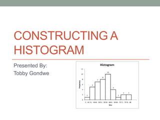
16. Step Five Continues
Draw the Histogram

17. Conclusion
• This is how we can construct or create a histogram given
a data set.
Exercise
Construct a histogram using the following data set.
Weekly wage Frequency
15 – 19 8
20 - 24 10
25 - 29 16
30 - 34 25
35 - 39 14
40 - 44 7

18. The End!
• Thank you!