Chapter11 economics

Elec3017:
Electrical Engineering Design
Chapter 11: Economics and Costing
A/Prof David Taubman
September 5, 2006

1 Purpose of this Chapter
In Chapter 3 we discussed product pricing and its interaction with costing. In
this chapter we begin by considering methods to develop reasonable cost esti-
mates for a new product. Together with a selling price and marketing estimates
of the expected sales volume, we will then be in a position to build a business
plan for our product development activity. This is the subject of Section 3,
in which we develop an economic framework for making product development
decisions. We conclude the chapter in Section 4, with a brief discussion of non-
economic factors, which should also be taken into consideration when making
decisions.

2 Elements of a Costing System
If a manufacturing company were to produce only one product, and all costs
were directly proportional to the number of units of that product produced,
costing would be a relatively simple process. There are several things which
make costing difficult. One of these is the fact that many manufacturing costs
are shared across multiple products. Examples include rent, lease or deprecia-
tion on machinery, and development costs which might not even contribute to
saleable products (e.g., aborted development projects). Another source of diffi-
culty is that certain costs may be difficult to reliably anticipate: manual labour
requirements may be hard to predict; foreign exchange rates may fluctuate; and
so forth.
To address these difficulties, it is helpful to identify two separate elements
of a costing system. The first is a cost accumulation system (i.e., an accounting
system), which keeps track of all actual costs, classifying them according to
the nature of the activity. The second element is a set of cost cost objectives.
In our case, the cost objectives are the manufactured products from which we
expect to derive our revenue. At the end of the day, our goal is to attribute

1

c
°Taubman, 2006 ELEC3017: Economics and Costing Page 2

electronic components
Cost objectives
unpopulated PCB
(outsourced)
Product A
Accumulated dedicated product
direct costs testing staff

package & shipping

product promotion

materials handling

component insertion
machinery Product B

Accumulated soldering machinery
indirect costs
rent & utilities

managerial staff

new product development

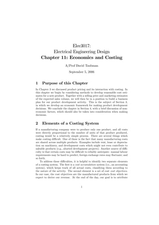
Figure 1: Attributing accumulated costs to cost objectives (products). Listed
costs are for illustrative purposes only. Dashed lines are used to highlight the
fact that indirect costs can only be approximately assigned to cost objectives.
This is done through “cost drivers.”

all accumulated costs to cost objectives. This includes not only those costs
which are directly related to the products we manufacture, but also indirect
costs (overhead). This allocation of costs to objectives is illustrated in Figure
1.
As suggested by the figure, direct costs and indirect costs need to be treated
differently. Direct costs are those which are incurred as a direct result of man-
ufacturing a specific product. Examples include the cost of purchasing compo-
nents, the cost of packaging and shipping products, and the direct labour costs
associated with personnel who work solely on the production a single product.
All other costs are indirect, and a meaningful basis must be found for attributing
these indirect costs to products; this is the subject of Section 2.2 below.
The reason for attributing all costs to products (cost objectives) is that these
are the only means we have of recovering our costs. In order to determine the
profitability of a new product development effort, it is important to ascertain
the degree to which profits will eventually outstrip costs. If we do not account
correctly for all costs, applying our resources to seemingly profitable products
may leave us bankrupt.

c

2.1 Direct Costs
The most obvious example of a direct cost is the cost of the various components
found on our product’s BOM (Bill of Materials). At a simplistic level, we can
say that this cost is directly proportional to the number of product units which
we manufacture and sell. In practice, of course, the cost of components will
vary with the quantity in which we buy them, but this can readily be factored
into the costing model for the new product we are developing.
More generally, any cost which can be directly related to the number of
produced units of a particular product is best considered a direct cost. Figure 1
shows some other examples. In some cases, costs associated with personnel can
be considered direct. This is true if a product requires dedicated staff (direct
labour), whose resources cannot be shared with other products. One approach is
to identify permandent internal staff as indirect costs, and external contractors
or casual workers as direct costs.

2.2 Indirect Costs and Cost Drivers
Many of the accumulated costs associated with running an organization cannot
be directly allocated to individual products. Examples include:

• Senior managers, supervisors, office staff, maintenance and cleaning staff;
• Depreciation or lease of manufacturing equipment;
• Rent, utilities (e.g., electricity) and insurance;
• Computers, photocopiers and office consumables;
• Staff development training;
• The costs of aborted development efforts.

One way to handle indirect costs is to factor them into an overhead margin.
This can only be done based on experience. Over time, for example, we may
find that our indirect costs average out at around $5,000,000 per year and that
our direct manufacturing costs for revenue generating products typically come
to around $20,000,000 per year. Based on this information, we determine that
a 25% margin should be added to the direct costs of every product, in order to
cover indirect costs. This overhead margin is added prior to any profit margin.
This method is very simple, but does not properly reflect the impact of design
decisions on costs. In particular, this method provides no incentive to develop
new products which place less demand on expensive manufacturing machinery,
require less labour supervision, and so forth. The margin approach also fails to
recognize the impact of sales volume on the per-unit costs of a product.
For these reasons, it is desirable to more carefully attribute at least some of
the indirect costs to specific products and the number of units of these products
which we expect to manufacture. In this context, we introduce the notion
of a cost driver. A cost driver is any factor which affects the cost of other

c

activities. For example, component handling costs are affected by the number
of components which must be handled. The cost driver in this case is the number
of components. Depreciation or leasing costs for manufacturing machinery are
affected by the amount of operating time consumed in manufacturing each unit
of a product1 . This, in turn, can usually be decomposed into more detailed
cost drivers, such as the number of components which an insertion machine
must insert into our product’s PCB. Again, the cost driver here might simply
be number of components, although more complex examples will be considered
in lectures.
If an activity has only one cost driver, the accumulated costs associated with
that activity can be simply converted into a costs per unit of the relevant cost
driver. For example, if component handling labour costs amount to $300,000
per annum (based on experience), and our component handling staff typically
order, receive, sort and load 5,000,000 components per annum (also based on
experience), the cost of these activity is identified as $0.06/component. This
can then be attributed to the cost of each unit of a product under development,
simply by multiplying the number of components in that product by $0.06. Of
course, the method is far from perfect. If we are a small firm, with too many
materials handling personnel, they have time on their hands so it will not cost
us anything extra if we manufacture more units of a product — it will simply
give them more work to do. The cost driver method essentially assumes that
are able to efficiently use our resources.
There can, of course, be multiple cost drivers for an activity. For example, a
machine might be capable of performing component insertion and wave soldering
in a tight pipeline. We can convert the annual leasing costs of this machine to
an hourly rate, based on an assumed operating schedule. However, the amount
of time taken to manufacture a unit of our product depends on which of the two
pipelined operations takes longer. If our product has a lot of components, so
that component insertion takes longer than wave soldering, the amount of time
taken to process a unit of the product depends on the number of components,
which becomes the cost driver. On the other hand, if the number of components
is small, wave soldering might dominate so that the cost driver is the number
of PCB’s2 . In this case, each cost driver has an associated per-unit cost (per-
component or per-PCB in our example), but only one cost driver is applicable,
depending on the design.
In the end, a mixture of direct costing, cost drivers and naive overhead
margins are used to attribute all costs to cost objectives (products). Direct
costing is used where possible. For the remaining indirect costs, cost drivers
should be identified where possible. Finally, all remaining indirect costs are
covered by a single overhead margin.
1 The reasoning here, is that if we need to operate a particular type of manufacturing
equipment for twice as much time, we probably need to lease or purchase (and depreciate)
twice as many machines. At least this is true if our manufacturing operation is big enough to
fully consume the resources that we have available.
2 For wave soldering, each PCB takes the same amount of time to solder, no matter how

many components it holds.

c

2.3 Costing your ELEC3017 Design Project
For your ELEC3017 design project, you are required to estimate manufactur-
ing costs. In a real production environment, costing is a careful activity which
strives to achieve accurate outcomes. Quotes from third party manufacturer’s
are obtained and converted to firm contracts. Labour and machine time require-
ments are calculated from detailed knowledge of the design and close interaction
with manufacturing managers. The level of accuracy required depends on your
expected profit margin. For high volume commodity products, profit margins
may be little than 10%, so costing must be very accurate to avoid the possibil-
ity that the product loses money. For lower volume, specialty products, profit
margins may exceed 100%, which reduces the burden on accurate costing.
Even in real product development, accurate costing is not achieved all at
once. During the early design phases, rough estimates are all that is possible.
This is reflected in your own design proposal, for which estimates will be based
mainly around critical components. For your final report, costing should be
much more thorough. The costing procedures you should use are itemized below.
Note carefully, however, that these are all manufacturing costs. They do not
include any profit margin for the manufacturer; nor do they include margins
added by retailers. For more on such matters, refer to the general discussion of
pricing strategies in Chapter 3.

2.3.1 Electronic Components
If possible, obtain the wholesale price for quantities of 1000 or 10,000 at a time
from manufacturers’ web-sites. If you cannot do this, divide the price you pay
for components from an electronics store such as Jaycar, Altronics or RS Farnell
by about 4. As an example, you should find that individual resistors cost about
$0.01 each, while small ceramic capacitors cost around $0.02 each.

2.3.2 Printed Circuit Board
Most projects will require one PCB. For the sake of uniformity, you should price
the PCB at $2.00, plus $0.01 for each IC pin and passive component lead. This
last cost could be understood as a drilling cost, but many components employed
in final designs may use surface mount technology. It is better understood as a
way of reflecting the impact of design complexity on the size of the PCB. These
costs include the soldering of components onto the PCB.

2.3.3 Mechanical Enclosures
The easiest way to price mechanical enclosures is to find a suitable plastic or
metal case from an electronics hobby store and divide their price by 4. You
may, however, have a more reliable means to estimate such costs — be sure to
justify whatever method you choose.

c

2.3.4 Component Handling and Insertion Costs
Assume that the combined handling and insertion costs associated with each
component amount to $0.25. The only exception to this is resistors and ca-
pacitors, whose handling and insertion costs should be estimated as $0.10 each.
Note that this may provide you with an incentive to use resistor or capacitor
networks in your final design. The cost of handling and inserting networks is to
be quoted as $0.25 each (as for IC’s), but each network typically includes 4 or
more individual components.

2.3.5 Packaging and Shipping of the Product
For simplicity, assume that packaging, handling and shipping of the final product
costs (k + 1) dollars, where k is the expected weight of your final product, in
kilograms.

2.3.6 Overhead Margin
To accommodate all other indirect costs, add a 20% margin to the costs identi-
fied above — i.e., everything from components through to packaging and shipping
costs.

2.3.7 Personnel
For your final report, you need to include the cost of development activities
leading up to manufacture and sale of your product. To that end, you should
estimate the total cost of each design engineer to be $120/hour. This is intended
to include salary, payroll tax, superannuation, office space occupied by the engi-
neer, ongoing staff development training, and the cost of related administrative
support. This cost is not subject to any additional overhead margin.

3 Cash Flow and the Time Value of Money
Product design and development can (and should) be understood as a finan-
cial investment. During the development phases, financial resources (materials,
salaries and overheads) must be invested. During the initial phases of commer-
cialization, cash outflows also exceed inflows. Components must be purchased,
manufactured product stock must be accumulated and product must be distrib-
uted to retail chains before any financial return can be expected. In the long
run, you hope that cash inflows from sale of the product will exceed your cash
outflows. Figure 2 illustrates the cumulative outward (-ve) and inward (+ve)
cash flows associated with a typical product, starting from design and running
through to the point when the market becomes saturated so that sales drop to
zero. Cash flows such as these are the main features of a business plan.
Since cash outflow precedes cash inflow, we have to be careful to account for
the time value of money. If I spend $1000.00 today and recoup $1000 one year

c

Cumulative inflow/outflow

Development costs
Ramp-up costs
Marketing and
support costs
Production costs

Figure 2: Cash flow for a typical product life cycle.

later, this is not a break even proposition. The $1000 I recoup in the future is
worth less than the $1000 I spend today. One way to understand this is that
inflation has degraded the value of my money. Another way to understand it
is that I could have invested the original $1000 safely in a bank and earned
interest, doing nothing in return. Thus, to consider that an investment breaks
even, I need at least to recover the interest that I might otherwise have earned.
There are, of course, a variety of more complex factors that should be con-
sidered in a sound business plan. Spending money today for a reward tomorrow
involves risk. New product development is certainly a more risky enterprise than
investing money in a bank. The market dynamics may change over time, foreign
exchange rates may adversely impact both selling price and costs, competitors
may emerge, and unexpected technical difficulties might be encountered. There
could also be unexpected legal liabilities. In view of these risks, we should ex-
pect a higher rate of return on our product development investment than the
interest offered by banks.
In the following sub-sections, we discuss ways of evaluating and expressing
the profitability of a product development activity, so that it can be compared
with other forms of investment. You may also refer to Ulrich and Eppinger [1,
Chapter 11] for a discussion of these issues.

3.1 Net Present Value (NPV)
As mentioned above, a dollar today is generally worth more than a dollar tomor-
row — just how much more depends on the assumed discount rate, r. You can
think of r as the annual compound interest rate paid by a reference investment
scheme. For your product development activity to break even, it must achieve
the same performance as this reference investment scheme. This means that
Y dollars, earned t years in the future, will exactly offset an expenditure of X

c

dollars today so long as
³ r ´t
Y =X · 1+
100
This is just the compound interest formula, with r expressed as an annual
percentage rate.
Following this argument, we may convert any future revenue Y (t) into an
equivalent value Y (0), measured in today’s dollars, according to

Y (t)
Y (0) = ¡ ¢
r t
1+ 100

The same may be done for future expenses, in which case Y (t) and Y (0) are
negative quantities. We say that Y (0) is the Present Value (PV) of the future
cash inflow or outflow Y (t), at time t.
We have said that our product development investment will break even if
it performs as well as a safe reference investment, paying interest rate r. An
equivalent way to express this break even condition is that the PV of all future
revenue minus the PV of all future expenses equals 0; that is, the Net Present
Value (NPV) of all future cash flows equals 0.

3.2 Ways of Expressing Profitability
One way to express the profitability of a development investment is to simply
measure the NPV of all future cash flows, based on an assumed discount rate
r. This is somewhat useful, but it does not tell us how sensitive the NPV is to
our selected value for r.
In practice, it is hard to know exactly what value for r is most appropriate.
A more interesting question than the magnitude of the NPV, therefore, is the
value of r at which the NPV becomes 0. This value is known as the Return
on Investment (ROI). The ROI allows us to compare our product development
activity with other forms of investment. An ROI of 7% is probably not all that
attractive if lower risk investments such as bank deposits are paying interest at
a rate of 6%.
Another method which is sometimes used to express profitability is the pay-
back period. This is the period P , such that the NPV of all cash flows prior to
time P is zero. The payback period is primarily of interest in identifying risk.
A development activity with a payback period of 20 years exposes us to a lot of
risk, since it is hard to predict cash flows with any reliability that far into the
future. Quite often, the payback period is evaluated at a discount rate of r = 0.
While this reduces its validity somewhat, the actual value of r has only a small
impact on short payback periods.

3.3 Economic Decision Making and Sunk Costs
The purpose of cash flow analysis is ultimately to help us make informed deci-
sions. As part of the ongoing process of planning, project managers must weigh

c

Internal Factors
• Research and Product External Factors
development costs • Product price
• Development time
Development • Sales volume
• Production costs Project • Competition
• Product performance

Product profit
(net present value)

Figure 3: Factors affecting product profitability.

the consequences of investing more (or less) development time, adding (or re-
moving) product features, using more (or less) expensive components, and so
forth. Each of these decisions has an impact on expected future cash flows and
hence profitability.
For example, if more features are added, the product will become more costly
to manufacture, but marketing intelligence may suggest that this will be more
than offset by increased product attractiveness, leading to a higher selling price
and/or a larger market volume. On the other hand, adding more features to
the product requires a larger up front investment in development, with a longer
development period. NPV analysis shows that the ROI is nevertheless improved
by the addition of more features, although the payback period is increased,
exposing us to more risk. This type of analysis (with hard numbers) is exactly
what management needs, to determine whether or not the decision to add more
features should be taken.
Figure 3 illustrates some of the different types of factors which can influence
profitability of a product development activity. Some of these factors (the in-
ternal ones) are at least partly under our control; others are outside our control,
but still need to be taken into account. Considering the many factors which
influence product profitability, economic analysis provides us with a framework
for making good decisions. By computing NPV, ROI and payback period under
a range of different scenarios, it is possible to understand the potential benefits
and risks of a various design decisions.
In other words, the purpose of economic analysis is to answer “what if” ques-
tions. The answers to these questions are not often obvious, due to conflicting
factors. Figure 4 illustrates the conflicting implications of the internal factors
identified in Figure 3. For example, product performance can generally be en-
hanced by increasing development time, increasing development costs (e.g., by
involving more personnel), and/or including higher quality components. Devel-
opment costs and higher performing components both add to the product cost.
On the other hand, it may be possible to decrease the product cost, without
sacrificing performance, by investing more time in development to come up with
efficient designs.
Perhaps the most important decision of all to be made with the help of

c

reduce
Development Time Product Cost

increase increase

increase
Product Performance Development Cost

Figure 4: Complex interaction between internal factors over which we have con-
trol.

economic analysis is whether the product development activity should proceed or
not. These so-called “go/no-go” decisions are typically taken at several points,
such as:

1. during an initial design review, shortly after concept generation;
2. once an initial functional prototype has been constructed; and
3. prior to manufacturing ramp-up.

Like all planning decisions, go/no-go decisions should be forward looking.
The fact that we have already spent $10,000,000 developing a revolutionary new
product should not in itself either positively or negatively influence our decision
to proceed (or not to proceed) with the development. All such previous expendi-
ture (and revenue, if any) is known as sunk costs. All we are interested in, from
a rational economic perspective, are future expenses and returns. This is why
NPV is computed based only on future cash flows, converted to present values;
previous cash flows are not relevant. More likely than not, previous expendi-
ture has brought us closer to finalizing the development activity so that future
costs are lower than they were at the start. As a result, each time we review
our economic forecasts, we would normally expect NPV and ROI to increase,
while the payback period decreases, making it progressively less likely that we
will take the decision not to proceed. Nevertheless, it is always possible that
changed circumstances render the activity unprofitable from a forward looking
perspective. When that happens, you should resist the gambler’s compulsion to
recoup sunk costs by plunging blindly on.

4 Non-Economic Considerations
Based on the foregoing discussion, one might conclude that economic merit is
the only sound basis for product development decisions. The reality, however,
is much more complex. First, we should remember that economic indicators
such as NPV are based on estimates of future cash flows, which are far from
perfect. The fact that we can compute answers to 2 decimal places should not

c

Qualitative factors specific to your company

know best
what you
– ability to leverage design experience for future products
– degree to which product fits long term strategic objectives
– impact on employee morale
– impact on stock price and credit rating
– risk in relation to the company’s financial resources

Qualitative factors in your target market
– expected reaction of competitors to your products
– impact on the brand-name perception amongst consumers

Qualitative factors in the socio-economic environment
know least
what you

– impact of potential changes in consumer buying power
– impact of government regulations
– impact of social trends and expectations of consumers

Figure 5: Various qualitative factors to supplement economic factors as a basis
for product development decisions.

fool us into thinking that they are any more accurate than the underlying data
on which they are based. Indeed, an analysis should normally be conducted to
determine how sensitive our NPV, ROI or payback period conclusions are to the
most critical underlying assumptions. A simple way to do this is just to re-run
the calculations under a variety of different scenarios.
Sometimes, the time and effort required to carefully estimate future cash
flows can get out of hand, detracting from the core business of design. This can
lead to lost productivity and perhaps missing a window of opportunity. Like
all aspects of design, therefore, we must be prepared to accept a compromise
between the quality of the information we have and the need to bring a successful
product to market quickly. Simply put, there needs to be an appropriate balance
between the effort spent planning and forecasting and the effort spent actually
doing the work of design.
Beyond money itself, there are a number of more qualitative factors which
should be factored into product development decisions. From a strategic per-
spective, it may make sense to pursue an economically unprofitable development
activity, because we expect that it will help us to capture a segment of the mar-
ket which we can exploit with future, more profitable products. From a human
resources perspective, it may make sense to continue a development activity in
which engineers have already invested a large amount of design effort, so as to
avoid low morale. Low morale may lead to the loss of experienced personnel
to our competitors, along with their accumulated technical knowledge. Figure
5 provides a more extensive list of qualitative factors which may need to be

c

factored into decision making processes.

References
[1] Ulrich, K. T. and Eppinger, S. D., Product Design and Development 2 ed ,
McGraw Hill, 2000.

Chapter11 economics

Recommandé

Recommandé

Contenu connexe

Tendances

Tendances (16)

En vedette

En vedette (20)

Similaire à Chapter11 economics

Similaire à Chapter11 economics (20)

Plus de Vin Voro

Plus de Vin Voro (20)

Dernier

Dernier (20)

Chapter11 economics