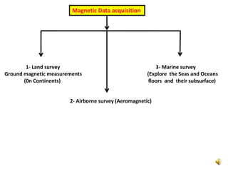
1. Magnetic Data acquisition
1- Land survey
Ground magnetic measurements
(0n Continents)
2- Airborne survey (Aeromagnetic)
3- Marine survey
(Explore the Seas and Oceans
floors and their subsurface)
3. The magnetic method has thus expanded from its initial use solely as a tool for finding iron
ore to a common tool used in exploration for minerals, hydrocarbons, ground water, and
geothermal resources. The method is also widely used in applications other than exploration,
such as studies focused on water-resource assessment (Smith and Pratt, 2003; Blakely et al.,
2000a), environmental contamination issues (Smith et al., 2000), seismic hazards (Blakely et al.,
2000b; Saltus et al., 2001; Langenheim et al., 2004), park stewardship (Finn and Morgan, 2002),
geothermal resources (Smith et al., 2002), volcano-related landslide hazards (Finn et al., 2001),
regional and local geologic mapping (Finn, 2002), mapping unexploded ordnances (Butler, 2001;
Hansen et al., 2005), locating buried pipelines (McConnell et al., 1999), archeological mapping
(Tsokas and Papazachos, 1992), and delineating impact structures (Campos-Enriquez, et al.,
1996; Goussev et al., 2003), which can sometimes be of economic importance (Mazur et al.,
2000).
Economic Importance of The Magnetic Method
4. Aeromagnetic or airborne survey
Aeromagnetic or airborne survey is most common among magnetic surveys. This is due to
the fact that it is rapid and cost effective. Besides, large areas can be surveyed easily without the
cost of sending a field party into the survey area and data can be obtained from areas
inaccessible to ground survey. Usually in aeromagnetic survey, data are obtained at stations
along series of parallel primary flight lines at a fixed spacing. Ideally the spacing is about one-
half the distance between the aeroplane and the basement [9]. The primary lines are tied by
cross-line at greater distances forming rectangles with common dimensions of 1 Km by 6 Km, 2
Km by 10 Km
A typical flight plan for an aeromagnetic survey.
5. WHAT ARE THE ADVANTAGES OF AN AEROMAGNETIC GEOPHYSICAL SURVEY?
There are many different types of aeromagnetic geophysical surveys: magnetic, radiometric,
electromagnetic, gravimetric and fixed onto a wing. These surveys make it possible to effectively
cover large areas that may be inaccessible or even dangerous without requiring any line cutting,
thereby dramatically reducing overhead so that costs are lower than those of any geophysical
land survey for a large area. However, the resolution they provide is lower than that of
terrestrial geophysical surveys. Generally, an airborne magnetic survey can not accurately locate
drill targets.
6. Fig. 1 The survey geometry , requires definition of three key parameters:
the survey line spacing and orientation and the flight height.
7. Survey design
Sampling theory requires individual measurements of TMI to be spaced at a maximum of
half the wavelength of the shortest wavelength of variation. Economic and safety factors mean
this is rarely practical and some aliasing of responses is the norm. This is not necessarily a
major problem since during qualitative interpretation of the data it is relative changes in
amplitude and texture that are used, and in fact accurate definition of the variations is only
required when specific anomalies need to be analyzed quantitatively (see Magnetic
Anomalies, Interpretation) and often there is a follow-up, more detailed, survey of the area of
interest to improve anomaly characterization.
Survey specifications
The survey geometry, illustrated in Figure 1, requires definition of three key parameters:
the survey line spacing and orientation and the flight height. Typical values of two of these
variables for different survey types are given in Table 1. Note that the tie-line spacing is a
dependent variable, typically being set to ten times the survey line spacing, although this may
be reduced to five times or less for high resolution surveys. The survey line spacing controls
the cost of the survey, which for fixed-wing aircraft is based on the total length of lines flown.
The total line length of a survey in terms of the survey area and line spacing can be estimated
from the equation below (Brodie, 2002).
8. Where ΔSurvey lines and ΔTie lines are the survey- and tie line spacings in meters, respectively,
the total line length is in kilometers, and the survey area is in square kilometers.
To this cost must be added nonproduction costs such as mobilization and “stand by” costs
associated with factors outside the acquisition company’s control, for example, bad weather,
magnetic storms. With helicopter surveys the time spent in the air is also taken into account,
and may be significant in mountainous areas where weather conditions severely restrict data
acquisition both in terms of flying time and location (Mudge, 1996).
9. Today, high-resolution aeromagnetic surveys, or HRAM surveys, are considered industry
standard, although exactly what flight specifications constitute a high-resolution survey are ill-
defined. Typical exploration HRAM surveys have flight heights of 80-150 m and line spacings of
250-500 m (Millegan, 1998). Exploration surveys are generally flown lower in Australia, at 60-80
m above ground (e.g., Robson and Spencer, 1997), and even lower if acquired by the Geological
Survey of Finland (30-40 m flight height with 200-m line spacing. Airspace regulations, urban
development, or rugged terrain prevent such low-altitude flying in many places. In contrast to
these typical exploration specifications, aeromagnetic studies that require high resolution of
anomalies in plan view, such as those geared toward mapping complicated geology, usually
entail uniform line spacings and flight heights, following the guidelines established by Reid
(1980).
10.
11. Basic Sensor Configurations
1- Towed bird installation
2- Tail-stinger installation
3- Wing tip mounting
Airborne Data collection
Airborne can be performed using:
- Fixed wing - Rotary-wing
aircraft (helicopter) aircraft
-Tend to be highly magnetic.
-Semi-detailed work and in rugged
terrain.
- Under normal circumstances, F.W. are
less expensive, cover an area faster, and
produce higher quality data (less noisy),
higher sensitivity results.
27. Diagram o f airborne magnetic survey and sources of anomalies with cross-section
and corresponding magnetic profile above
The Sharp colosur at the near edge is from a
dike-like body
28. For any of the airborne magnetometer systems. the instrument assembly in the airplane
carries the necessary electronics and a recorder on which a continuous record of the magnetic
field is shown. The airplane also usually is equipped with a radar altimeter and with the
necessary positioning equipment. The several items of data (magnetic field intensity,
electronic or photographic positioning data, barometric elevation, and height above ground)
are correlated with one another so that all can be brought together to provide the necessary
information for reducing the observations to a magnetic map.
29. a recorder on which a continuous record of the magnetic field is shown.
30. 2- Leveling (Tieing) Procedure to minimize (addition in airborne Survey)
Survey Lines
Tie Lines (wider spacing)
Magnetic Data correction Includes:
1- Fcorr = Fobs. – Fbase st. + IGRF ± Instrument drift (as in ground Survey),
32. Aeromagnetic Survey in Afghanistan
Afghanistan Composite Magnetic Anomaly Map at 5000 m Above Ground
33.
34. Aeromagnetic surveys are flown with a wide variety of terrain clearances. sampling rates, and
line spacings. The results are generally presented as contour maps, implying that the survey
grid defines the continuous magnetic field sufficiently well to justify interpolation.
35. 2- Marine Magnetic surveying
Marine survey is similar to those of aeromagnetic or airborne survey. The magnetic sensor is
towed in a housing known as ‘fish’ which is far behind the vessel (at least 2.5 ship’s length) to
remove its magnetic effects. Marine survey is very slow and is usually carried out in conjunction
with other geophysical methods, such as continuous seismic profiling and gravity surveying
(Keary and Brooks, 1988).
47. New Bedford, Massachusetts, USA - June 2, 2018: Geophysical survey vessel Ocean Researcher
crossing Acushnet River with New Bedford waterfront in background
48. Magnetic survey tracklines (total 107 line km). No data were acquired within the inner harbour
area due to high magnetic gradients associated with the modern harbour entranceway.