Supervised Corpus-based Methods for Word Sense Disambiguation

Chapter 7
SUPERVISED METHODS
Lluís Màrquez*, Gerard Escudero*, David Martínez♦, German Rigau♦
*Universitat Politècnica de Catalunya UPC ♦Euskal Herriko Unibertsitatea UPV/EHU
Abstract: In this chapter, the supervised approach to Word Sense Disambiguation is
presented, which consists of automatically inducing classification models or
rules from annotated examples. We start by introducing the machine learning
framework for classification and some important related concepts. Then, a
review of the main approaches in the literature is presented, focusing on the
following issues: learning paradigms, corpora used, sense repositories, and
feature representation. We also include a more detailed description of five
statistical and machine learning algorithms, which are experimentally
evaluated and compared on the DSO corpus. In the final part of the chapter,
the current challenges of the supervised learning approach to WSD are briefly
discussed.
1. INTRODUCTION TO SUPERVISED WSD
In the last fifteen years, the empirical and statistical approaches have
increased their impact on NLP significantly. Among them, the algorithms
and techniques coming from the machine learning (ML) community have
been applied to a large variety of NLP tasks with a remarkable success and
they are becoming the focus of an increasing interest. The reader can find
excellent introductions to ML and its relation to NLP in Mitchell (1997), and
Manning & Schütze (1999) and Cardie & Mooney (1999), respectively.
The type of NLP problems initially addressed by statistical and machine
learning techniques are those of “language ambiguity resolution”, in which
the correct interpretation should be selected, among a set of alternatives, in a
particular context (e.g., word choice selection in speech recognition or

2 Chapter 7
machine translation, part-of-speech tagging, word sense disambiguation, co-
reference resolution, etc.). They are particularly appropriate for ML because
they can be seen as classification problems, which have been studied
extensively in the ML community.
More recently, ML techniques have also been applied to NLP problems
that do not reduce to a simple classification scheme. We place in this
category: sequence tagging (e.g., with part-of-speech, named entities, etc.),
and assignment of hierarchical structures (e.g., parsing trees, complex
concepts in information extraction, etc.). These approaches typically proceed
by decomposition of complex problems into simple decision schemes or by
generalizing the classification setting in order to work directly with complex
representations and outputs.
Regarding automatic WSD, one of the most successful approaches in the
last ten years is the ‘supervised learning from examples’, in which statistical
or ML classification models are induced from semantically annotated
corpora. Generally, supervised systems have obtained better results than the
unsupervised ones, as shown by experimental work and international
evaluation exercises such as Senseval (see Chapter 4). However, the
knowledge acquisition bottleneck is still an open problem that poses serious
challenges to the supervised learning approach for WSD.
The overall organization of the chapter is as follows. The next subsection
introduces the machine learning framework for classification. Section 2
contains a survey on the state-of-the-art in supervised WSD, concentrating
on topics such as: learning approaches, sources of information, and feature
codification. Section 3 describes five learning algorithms which are
experimentally compared on the DSO corpus. The main challenges posed by
the supervised approach to WSD are discussed in Section 4. Finally, Section
5 concludes and devotes some words to the possible future trends.
1.1 Machine learning for classification
The goal in supervised learning for classification consists of inducing
from a training set S, an approximation (or hypothesis) h of an unknown
function f that maps from an input space X to a discrete unordered output
space Y={1,…,K}.
The training set contains n training examples, S={(x1
,y1
),…, (xn
,yn
)},
which are pairs (x,y) where x belongs to X and y=f(x). The x component of
each example is typically a vector x=(x1,…,xm), whose components, called
features (or attributes), are discrete- or real-valued and describe the relevant
information/properties about the example. The values of the output space Y
associated with each training example are called classes (or categories).

7. SUPERVISED METHODS 3
Therefore, each training example is completely described by a set of
attribute-value pairs, and a class label.
In the Statistical Learning Theory field (Vapnik 1998), the function f is
viewed as a probability distribution P(X,Y) and not as a deterministic
mapping, and the training examples are considered as a sample (independent
and indentically distributed) from this distribution. Additionally, X is usually
identified as ℜn
, and each example x as a point in ℜn
with one real-valued
feature for each dimension. In this chapter we will try to maintain the
descriptions and notation compatible with both approaches.
Given a training set S, a learning algorithm induces a classifier, denoted
h, which is a hypothesis about the true function f. In doing so, the learning
algorithm can choose among a set of possible functions H, which is referred
to as the space of hypotheses. Learning algorithms differ in which space of
hypotheses they take into account (e.g., linear functions, domain partitioning
by axis parallel hyperplanes, radial basis functions, etc.) in the representation
language used (e.g., decision trees, sets of conditional probabilities, neural
networks, etc.), and in the bias they use for choosing the best hypothesis
among several that can be compatible with the training set (e.g., simplicity,
maximal margin, etc.).
Given new x vectors, h is used to predict the corresponding y values, that
is, to classify the new examples, and it is expected to be coincident with f in
the majority of the cases, or, equivalently, to perform a small number of
errors. The measure of the error rate on unseen examples is called
generalization (or true) error. It is obvious that the generalization error
cannot be directly minimized by the learning algorithm since the true
function f, or the distribution P(X,Y), is unknown. Therefore, an inductive
principle is needed. The most common way to proceed is to directly
minimize the training (or empirical) error, that is, the number of errors on
the training set. This principle is known as Empirical Risk Minimization, and
gives a good estimation of the generalization error in the presence of
sufficient training examples. However, in domains with few training
examples, forcing a zero training error can lead to overfit the training data
and to generalize badly. The risk of overfitting is increased in the presence
of outliers and noise (i.e., very exceptional and wrongly classified training
examples, respectively). A notion of complexity of the hypothesis function
h, defined in terms of the expressiveness of the functions in H, is also
directly related to the risk of overfitting. This complexity measure is usually
computed using the Vapnik-Chervonenkis (VC) dimension (see Vapnik
(1998) for details). The trade-off between training error and complexity of
the induced classifier is something that has to be faced in any experimental
setting in order to guarantee a low generalization error.

4 Chapter 7
An example on WSD. Consider the problem of disambiguating the verb to
know in a sentence. The senses of the word know are the classes of the
classification problem (defining the output space Y), and each occurrence of
the word in a corpus will be codified into a training example (xi
), annotated
with the correct sense. In our example the verb know has 8 senses according
to WordNet 1.6. The definition of senses 1 and 4 are included in Figure 7-1.
Sense 1: know, cognize. Definition: be cognizant or aware of a fact or a specific
piece of information. Examples: "I know that the President lied to the people";
"I want to know who is winning the game!"; "I know it's time".
Sense 4: know. Definition: be familiar or acquainted with a person or an object.
Examples: "She doesn't know this composer"; "Do you know my sister?" "We
know this movie".
Figure 7-1. Sense definitions of verb know according to WordNet 1.6.
The representation of examples usually includes information about the
context in which the ambiguous word occurs. Thus, the features describing
an example may codify the bigrams and trigrams of words and POS tags
next to the target word and all the words appearing in the sentence (bag-of-
words representation). See Section 2.3 for details on example representation.
A decision list is a simple learning algorithm that can be applied in this
domain. It acquires a list of ordered classification rules of the form: if
(feature=value) then class. When classifying a new example x, the list of
rules is checked in order and the first rule that matches the example is
applied. Supposing that such a list of classification rules has been acquired
from training examples, Table 7-1 contains the set of rules that match the
example sentence: There is nothing in the whole range of human experience
more widely known and universally felt than spirit. They are ordered by
decreasing values of a log-likelihood measure indicating the confidence of
the rule. We can see that only features related to the first and fourth senses of
know receive positive values from its 8 WordNet senses. Classifying the
example by the first two tied rules (which are activated because the word
widely appears immediately to the left of the word know), sense 4 will be
assigned to the example.
Table 7-1. Classification example of the word know using Decision Lists.
Feature Value Sense Log-likelihood
±3-word-window “widely” 4 2.99
word-bigram “known widely” 4 2.99
word-bigram “known and” 4 1.09
sentence-window “whole” 1 0.91
sentence-window “widely” 4 0.69
sentence-window “known” 4 0.43

Finally, we would like to briefly comment a terminology issue that can
be rather confusing in the WSD literature. Recall that, in machine learning,
the term ‘supervised learning’ refers to the fact that the training examples are
annotated with the class labels, which are taken from a pre-specified set.
Instead, ‘unsupervised learning’ refers to the problem of learning from
examples when there is no set of pre-specified class labels. That is, the
learning consists of acquiring the similarities between examples to form
clusters that can be later interpreted as classes (this is why it is usually
referred to as clustering). In the WSD literature, the term ‘unsupervised
learning’ is sometimes used with another meaning, which is the acquisition
of disambiguation models or rules from non-annotated examples and
external sources of information (e.g., lexical databases, aligned corpora,
etc.). Note that in this case the set of class labels (which are the senses of the
words) are also specified in advance. See Section 1.1 of Chapter 6 for more
details on this issue.
2. A SURVEY OF SUPERVISED WSD
In this section we overview the supervised approach to WSD, focussing
on alternative learning approaches and systems. The three introductory
subsections address also important issues related to the supervised paradigm,
but in less detail: corpora, sense inventories, and feature design, respectively.
Other chapters in the book are devoted to address these issues more
thoroughly. In particular, Chapter 4 describes the corpora used for WSD,
Appendix X overviews the main sense inventories, and, finally, Chapter 8
gives a much more comprehensive description of feature codification and
knowledge sources.
2.1 Main corpora used
As we have seen in the previous section, supervised machine learning
algorithms use semantically annotated corpora to induce classification
models for deciding the appropriate word sense for each particular context.
The compilation of corpora for training and testing such systems requires a
large human effort since all the words in these annotated corpora have to be
manually tagged by lexicographers with semantic classes taken from a
particular lexical semantic resource—most commonly WordNet (Miller
1990, Fellbaum 1998). Despite the good results obtained, supervised
methods suffer from the lack of widely available semantically tagged
corpora, from which to construct broad-coverage systems. This is known as
the knowledge acquisition bottleneck. And the lack of annotated corpora is

6 Chapter 7
even worse for languages other than English. The extremely high overhead
for supervision (all words, all languages) explain why supervised methods
have been seriously questioned.
Due to this obstacle, the first attempts of using statistical techniques for
WSD tried to avoid the manual annotation of a training corpus. This was
achieved by using pseudo-words (Gale et al. 1992), aligned bilingual corpora
(Gale et al. 1993), or by working with the related problem of form
restoration (Yarowsky 1994).
Methods that use bilingual corpora rely on the fact that the different
senses of a word in a given language are translated using different words in
another language. For example, the Spanish word partido translates to match
in English in the sports sense and to party in the political sense. Therefore, if
a corpus is available with a word-to-word alignment, when a translation of a
word like partido is made, its English sense is automatically determined as
match or party. Gale et al. (1993) used an aligned French and English corpus
for applying statistical WSD methods with an accuracy of 92%. Working
with aligned corpora has the obvious limitation that the learned models are
able to distinguish only those senses that are translated into different words
in the other language.
The pseudo-words technique is very similar to the previous one. In this
method, artificial ambiguities are introduced in untagged corpora. Given a
set of related words, for instance {match, party}, a pseudo-word corpus can
be created by conflating all the examples for both words maintaining as
labels the original words (which act as senses). This technique is also useful
for acquiring training corpora for the accent restoration problem. In this case,
the ambiguity corresponds to the same word having or not a diacritic, like
the Spanish words {cantara, cantará}.
SemCor (Miller et al. 1993), which stands for Semantic Concordance, is
the major sense-tagged corpus available for English1
. The texts used to
create SemCor were extracted from Brown corpus (80%) and a novel, The
Red Badge of Courage (20%), and then manually linked to senses from the
WordNet lexicon. The Brown Corpus is a collection of 500 documents,
which are classified into fifteen categories. For an extended description of
the Brown Corpus see (Francis & Kučera 1982). The SemCor corpus makes
use of 352 out of the 500 Brown Corpus documents. In 166 of these
documents only verbs are annotated (totalizing 41,525 links). In the
remaining 186 documents all substantive words (nouns, verbs, adjectives and
adverbs) are linked to WordNet (for a total of 193,139 links).
DSO (Ng & Lee 1996) is another medium−big size semantically
annotated corpus. It contains 192,800 sense examples for 121 nouns and 70
verbs, corresponding to a subset of the most frequent and ambiguous English
words. These examples, consisting of the full sentence in which the
ambiguous word appears, are tagged with a set of labels corresponding, with

minor changes, to the senses of WordNet 1.5. Ng and colleagues from the
University of Singapore compiled this corpus in 1996 and since then it has
been widely used. The DSO corpus contains sentences from two different
corpora, namely the Wall Street Journal corpus (WSJ) and the Brown
Corpus (BC). The former focused on the financial domain and the second is
a general corpus.
Several authors have also provided the research community with the
corpora developed for their experiments. This is the case of the line-hard-
serve corpora with more than 4,000 examples per word (Leacock et al.
1998). The sense repository was WordNet 1.5 and the text examples were
selected from the Wall Street Journal, the American Printing House for the
Blind, and the San Jose Mercury newspaper. Another one is the interest
corpus2
with 2,369 examples coming from the Wall Street Journal and using
the LDOCE sense distinctions.
New initiatives like the Open Mind Word Expert3
(Chklovski & Mihalcea
2002) appear to be very promising (cf. Chapter 9). This system makes use of
the web technology to help volunteers to manually annotate sense examples.
The system includes an active learning component that automatically selects
for human tagging those examples that were most difficult to classify by the
automatic tagging systems. The corpus is growing daily and, nowadays,
contains more than 70,000 instances of 230 words using WordNet 1.7 for
sense distinctions. In order to ensure the quality of the acquired examples,
the system requires redundant tagging. The examples are extracted from
three sources: Penn Treebank corpus, Los Angeles Times collection (as
provided for the TREC conferences), and Open Mind Common Sense. While
the two first sources are well known, the Open Mind Common Sense corpus
provides sentences that are not usually found in current corpora. They
consist mainly in explanations and assertions similar to glosses of a
dictionary, but phrased in less formal language, and with many examples per
sense. The authors of the project suggest that these sentences could be a
good source of keywords to be used for disambiguation. The examples
obtained from this project were used in the English lexical-sample task in
Senseval-3.
Finally, resulting from Senseval international evaluation exercises, small
sets of tagged corpora have been developed for more than a dozen languages
(see Section 2.5 for details). The reader may find an extended description of
corpora used for WSD in Chapter 4 and Appendix Y.
2.2 Main sense repositories
Initially, machine readable dictionaries (MRDs) were used as the main
repositories of word sense distinctions to annotate word examples with
senses. For instance, LDOCE, the Longman Dictionary of Contemporary

8 Chapter 7
English (Procter 1978) was frequently used as a research lexicon (Wilks et
al. 1993) and for tagging word sense usages (Bruce & Wiebe 1994).
At Senseval-1, the English lexical-sample task used the HECTOR
dictionary to label each sense instance. This dictionary was produced jointly
by Oxford University Press and DEC dictionary research project. However,
WordNet (Miller 1991, Fellbaum 1998) and EuroWordNet (Vossen 1998)
are nowadays becoming the most common knowledge sources for sense
distinctions.
WordNet is a Lexical Knowledge Base of English. It was developed by
the Cognitive Science Laboratory at Princeton University under the direction
of Professor George Miller. Current version 2.0 contains information of
more than 129,000 words which are grouped in more than 99,000 synsets
(concepts or synonym sets). Synsets are structured in a semantic network
with multiple relations, the most important being the hyponymy relation
(class/subclass). WordNet includes most of the characteristics of a MRD,
since it contains definitions of terms for individual senses like in a
dictionary. It defines sets of synonymous words that represent a unique
lexical concept, and organizes them in a conceptual hierarchy similar to a
thesaurus. WordNet includes also other types of lexical and semantic
relations (meronymy, antonymy, etc.) that provide the largest and richest
freely available lexical resource. WordNet was designed to be
computationally used. Therefore, it does not have many of the associated
problems of MRDs (Rigau 1998).
Many corpora have been annotated using WordNet and EuroWordNet.
Since version 1.4 up to 1.64
Princeton provides also SemCor (Miller et al.
1993). DSO is annotated using a slightly modified version of WordNet 1.5,
the same version used for the line-hard-serve corpus. The Open Mind Word
Expert initiative uses WordNet 1.7. The English tasks of Senseval-2 were
annotated using a preliminary version of WordNet 1.7 and most of the
Senseval-2 non-English tasks were labeled using EuroWordNet. Although
using different WordNet versions can be seen as a problem for the
standardization of these valuable lexical resources, successful algorithms
have been proposed for providing compatibility across the European
wordnets and the different versions of the Princeton WordNet (Daudé et al.
1999, 2000, 2001).
2.3 Representation of examples by means of features
Before applying any ML algorithm, all the sense examples of a particular
word have to be codified in a way that the learning algorithm can handle
them. As explained in Section 1.2, the most usual way of codifying training

examples is as feature vectors. In this way, they can be seen as points in an n
dimensional feature space, where n is the total number of features used.
Features try to capture information and knowledge about the context of
the target words to be disambiguated. Computational requirements of
learning algorithms and the availability of the information impose some
limitations on the features that can be considered, thus they necessarily
codify only a simplification (or generalization) of the word sense instances
(see Chapter 8 for more details on features).
Usually, a complex pre-processing step is performed to build a feature
vector for each context example. This pre-process usually considers the use
of a windowing schema or a sentence-splitter for the selection of the
appropriate context (it ranges from a fixed number of content words around
the target word to some sentences before and after the target sense example),
a POS tagger to stablish POS patterns around the target word, ad-hoc
routines for detecting multi-words or capturing n-grams, or parsing tools for
detecting dependencies between lexical units.
Although this preprocessing step, in which each example is converted
into a feature vector, can be seen as an independent process from the ML
algorithm to be used, there are strong dependencies between the kind and
codification of the features and the appropriateness for each learning
algorithm (e.g., exemplar-based learning is very sensitive to irrelevant
features, decision tree induction does not properly handle attributes with
many values, etc.). Escudero et al. (2000b) discusse how the feature
representation affects both the efficiency and accuracy of two learning
systems for WSD. See also (Agirre & Martínez 2001) for a survey on the
types of knowledge sources that could be relevant for codifying training
examples.
The feature sets most commonly used in the supervised WSD literature
can be grouped as follows :
1. Local features, represent the local context of a word usage. The local
context features comprise n-grams of POS tags, lemmas, word forms and
their positions with respect to the target word. Sometimes, local features
include a bag-of-words or lemmas in a small window around the target
word (the position of these words is not taken into account). These
features are able to capture knowledge about collocations, argument-head
relations and limited syntactic cues.
2. Topic features, represent more general contexts (wide windows of words,
other sentences, paragraphs, documents), usually in a bag-of-words
representation. These features aim at capturing the semantic domain of
the text fragment or document.

10 Chapter 7
3. Syntactic dependencies, at a sentence level, have also been used to try to
better model syntactic cues and argument-head relations.
2.4 Main approaches to supervised WSD
We may classify the supervised methods according to the ‘induction
principle’ they use for acquiring the classification models. The one presented
in this chapter is a possible categorization, which does not aim at being
exhaustive. The combination of many paradigms is another possibility,
which is covered in Section 4.6. Note also that many of the algorithms
described in this section are lately used in the experimental setting of Section
3. When this occurs we try to keep the description of the algorithms to the
minimum in the present section and explain the details in Section 3.1.
2.4.1 Probabilistic methods
Statistical methods usually estimate a set of probabilistic parameters that
express the conditional or joint probability distributions of categories and
contexts (described by features). These parameters can be then used to
assign to each new example the particular category that maximizes the
conditional probability of a category given the observed context features.
The Naive Bayes algorithm (Duda et al. 2001) is the simplest algorithm
of this type, which uses the Bayes inversion rule and assumes the conditional
independence of features given the class label (see Section 3.1.1 below). It
has been applied to many investigations in WSD (Gale et al. 1992, Leacock
et al. 1993, Pedersen & Bruce 1997, Escudero et al. 2000b) and, despite its
simplicity, Naive Bayes is claimed to obtain state-of-the-art accuracy in
many papers (Mooney 1996, Ng 1997a, Leacock et al. 1998). It is worth
noting that the best performing method in the Senseval-3 English lexical
sample task is also based on Naive Bayes (Grozea 2004).
A potential problem of Naive Bayes is the independence assumption.
Bruce & Wiebe (1994) present a more complex model known as the
‘decomposable model’ which considers different characteristics dependent
on each other. The main drawback of this approach is the enormous number
of parameters to be estimated, proportional to the number of different
combinations of the interdependent characteristics. As a consequence, this
technique requires a great quantity of training examples. In order to solve
this problem, Pedersen & Bruce (1997) propose an automatic method for
identifying the optimal model by means of the iterative modification of the
complexity level of the model.
The Maximum Entropy approach (Berger et al. 1996) provides a flexible
way to combine statistical evidence from many sources. The estimation of

probabilities assumes no prior knowledge of data and it has proven to be
very robust. It has been applied to many NLP problems and it also appears as
a promising alternative in WSD (Suárez & Palomar 2002).
2.4.2 Methods based on the similarity of the examples
The methods in this family perform disambiguation by taking into account
a similarity metric. This can be done by comparing new examples to a set of
learned vector prototypes (one for each word sense) and assigning the sense
of the most similar prototype, or by searching in a stored base of annotated
examples which are the most similar and assigning the most frequent sense
among them.
There are many forms to calculate the similarity between two examples.
Assuming the Vector Space Model (VSM), one of the simplest similarity
measures is to consider the angle that both example vectors form (a.k.a.
cosine measure). Leacock et al. (1993) compared VSM, Neural Networks,
and Naive Bayes methods, and drew the conclusion that the two first
methods slightly surpass the last one in WSD. Yarowsky et al. (2001)
included a VSM model in their system that combined the results of up to six
different supervised classifiers, and obtained very good results in Senseval-2.
For training the VSM component, they applied a rich set of features
(including syntactic information), and weighting of feature types.
The most widely used representative of this family of algorithms is the k-
Nearest Neighbor (kNN) algorithm, which we also describe and test in the
experimental Section 3. In this algorithm the classification of a new example
is performed by searching the set of the k most similar examples (or nearest
neighbors) among a pre-stored set of labeled examples, and performing an
‘average’ of their senses in order to make the prediction. In the simplest
case, the training step reduces to store all of the examples in memory (this is
why this technique is called Memory-based, Exemplar-based, Instance-
based, or Case-based learning) and the generalization is postponed until each
new example is being classified (this is why it is sometimes also called Lazy
learning). A very important issue in this technique is the definition of an
appropriate similarity (or distance) metric for the task, which should take
into account the relative importance of each attribute and be efficiently
computable. The combination scheme for deciding the resulting sense
among the k nearest neighbors also leads to several alternative algorithms.
kNN-based learning is said to be the best option for WSD by Ng (1997a).
Other authors (Daelemans et al. 1999) argue that exemplar-based methods
tend to be superior in NLP problems because they do not apply any kind of
generalization on data and, therefore, they do not forget exceptions.

12 Chapter 7
Ng & Lee (1996) did the first work on kNN for WSD. Ng (1997a)
automatically identified the optimal value of k for each word improving the
previously obtained results. Escudero et al. (2000b) focused on certain
contradictory results in the literature regarding the comparison of Naive
Bayes and kNN methods for WSD. The kNN approach seemed to be very
sensitive to the attribute representation and to the presence of irrelevant
features. For that reason alternative representations were developed, which
were more efficient and effective. The experiments demonstrated that kNN
was clearly superior to Naive Bayes when applied with an adequate feature
representation and with feature and example weighting, and sophisticated
similarity metrics. Stevenson & Wilks (2001) also applied kNN in order to
integrate different knowledge sources, reporting high precision figures for
LDOCE senses (see Section 4.6).
Regarding Senseval evaluations, Hoste et al. (2001; 2002a) used, among
others, a kNN system in the English all words task of Senseval-2, with good
performance. At Senseval-3, a new system was presented by Decadt et al.
(2004) winning the all-words task. However, they submitted a similar system
to the lexical task, which scored lower than kernel-based methods.
2.4.3 Methods based on discriminating rules
These methods use selective rules associated with each word sense. Given
an example to classify, the system selects one or more rules that are satisfied
by the example features and assign a sense based on their predictions.
Decision Lists. Decision lists are ordered lists of rules of the form
(condition, class, weight). According to Rivest (1987) decision lists can be
considered as weighted if-then-else rules where the exceptional conditions
appear at the beginning of the list (high weights), the general conditions
appear at the bottom (low weights), and the last condition of the list is a
‘default’ accepting all remaining cases. Weights are calculated with a
scoring function describing the association between the condition and the
particular class, and they are estimated from the training corpus. When
classifying a new example, each rule in the list is tested sequentially and the
class of the first rule whose condition matches the example is assigned as the
result. Decision Lists is one of the algorithms compared in Section 3. See
details in Section 3.1.3.
Yarowsky (1994) used decision lists to solve a particular type of lexical
ambiguity: Spanish and French accent restoration. In a subsequent work,
Yarowsky (1995a) applied decision lists to WSD. In this work, each
condition corresponds to a feature, the values are the word senses and the

weights are calculated by a log-likelihood measure indicating the plausibility
of the sense given the feature value.
Some more recent experiments suggest that decision lists could also be
very productive for high precision feature selection for bootstrapping
(Martínez et al. 2002).
Decision Trees. A decision tree (DT) is a way to represent classification
rules underlying data by an n-ary branching tree structure that recursively
partitions the training set. Each branch of a decision tree represents a rule
that tests a conjunction of basic features (internal nodes) and makes a
prediction of the class label in the terminal node. Although decision trees
have been used for years in many classification problems in artificial
intelligence they have not been applied to WSD very frequently. Mooney
(1996) used the C4.5 algorithm (Quinlan 1993) in a comparative experiment
with many ML algorithms for WSD. He concluded that decision trees are not
among the top performing methods. Some factors that make decision trees
inappropriate for WSD are: (i) The data fragmentation performed by the
induction algorithm in the presence of features with many values; (ii) The
computational cost is high in very large feature spaces; and (iii) Terminal
nodes corresponding to rules that cover very few training examples do not
produce reliable estimates of the class label. Part of these problems can be
partially mitigated by using simpler related methods such as decision lists.
Another way of effectively using DTs is considering the weighted
combination of many decision trees in an ensemble of classifiers (see
Section 2.4.4).
2.4.4 Methods based on rule combination
The combination of many heterogeneous learning modules for developing
a complex and robust WSD system is currently a common practice, which is
explained in Section 4.6. In the current section, ‘combination’ refers to a set
of homogeneous classification rules that are learned and combined by a
single learning algorithm. The AdaBoost learning algorithm is one of the
most successful approaches to do it.
The main idea of the AdaBoost algorithm is to linearly combine many
simple and not necessarily very accurate classification rules (called weak
rules or weak hypotheses) into a strong classifier with an arbitrarily low
error rate on the training set. Weak rules are trained sequentially by
maintaining a distribution of weights over training examples and by updating
it so as to concentrate weak classifiers on the examples that were most
difficult to classify by the ensemble of the preceding weak rules (see Section
3.1.4 for details). AdaBoost has been successfully applied to many practical

14 Chapter 7
problems, including several NLP tasks (Schapire 2002) and it is especially
appropriate when dealing with unstable learning algorithms (e.g., decision
tree induction) as the weak learner.
Several experiments on the DSO corpus (Escudero et al. 2000a, 2000c,
2001), including the one reported in Section 3.2 below, concluded that the
boosting approach surpasses many other ML algorithms on the WSD task.
We can mention, among others, Naive Bayes, exemplar-based learning and
decision lists. In those experiments, simple decision stumps (extremely
shallow decision trees that make a test on a single binary feature) were used
as weak rules, and a more efficient implementation of the algorithm, called
LazyBoosting, was used to deal with the large feature set induced.
2.4.5 Linear classifiers and kernel-based approaches
Linear classifiers have been very popular in the field of information
retrieval (IR), since they have been successfully used as simple and efficient
models for text categorization. A linear (binary) classifier is a hyperplane in
an n-dimensional feature space that can be represented with a weight vector
w and a bias b indicating the distance of the hyperplane to the origin. The
weight vector has a component for each feature, expressing the importance
of this feature in the classification rule, which can be stated as: h(x)=+1 if
(w·x)+b ≥ 0 and h(x)=−1 otherwise. There are many on-line learning
algorithms for training such linear classifiers (Perceptron, Widrow-Hoff,
Winnow, Exponentiated-Gradient, Sleeping Experts, etc.) that have been
applied to text categorization—see, for instance, Dagan et al. (1997).
Despite the success in IR, the use of linear classifiers in the late 90’s for
WSD reduces to a few papers. Mooney (1996) used the perceptron algorithm
and Escudero et al. (2000c) used the SNoW architecture (based on Winnow).
In both cases, the results obtained with the linear classifiers were very low.
The expressivity of this type of classifiers can be boosted to allow the
learning of non-linear functions by introducing a non-linear mapping of the
input features to a higher-dimensional feature space, where new features can
be expressed as combinations of many basic features and where the standard
linear learning is performed. If example vectors appear only inside dot
product operations in the learning algorithm and the classification rule, then
the non-linear learning can be performed efficiently (i.e., without making
explicit non-linear mappings of the input vectors), via the use of kernel
functions. The advantage of using kernel-methods7
is that they offer a
flexible and efficient way of defining application-specific kernels for
exploiting the singularities of the data and introducing background
knowledge. Currently, there exist several kernel implementations for dealing

with general structured data. Regarding WSD, we find some recent
contributions in Senseval-3 (Strapparava et al. 2004, Popescu 2004).
Support Vector Machines (SVM), introduced by Boser et al. (1992), is
the most popular kernel-method. The learning bias consists of choosing the
hyperplane that separates the positive examples from the negatives with
maximum margin see (Cristianini & Shawe-Taylor 2000) and also
Section 3.1.5 for details. This learning bias has proven to be very powerful
and lead to very good results in many pattern recognition, text, and NLP
problems. The first applications of SVMs to WSD are those of Murata et al.
(2001) and Lee & Ng (2002).
More recently, an explosion of systems using SVMs has been observed
in the Senseval-3 evaluation (most of them among the best performing ones).
Among others, we highlight Strapparava et al. (2004), Lee et al. (2004),
Agirre & Martínez (2004a), Cabezas et al. (2004) and Escudero et al. (2004).
Other kernel-methods for WSD presented at Senseval-3 and recent
conferences are: Kernel Principal Component Analysis (KPCA, Carpuat et
al. 2004, Wu et al. 2004), Regularized Least Squares (Popescu 2004), and
Averaged Multiclass Perceptron (Ciaramita & Johnson 2004). We think that
kernel-methods are the most popular learning paradigm in NLP because they
offer a remarkable performance in most of the desirable properties: accuracy,
efficiency, ability to work with large and complex feature sets, and
robustness in the presence of noise and exceptions. Moreover, some robust
and efficient implementations are currently available.
Artificial Neural Networks, characterized by a multi-layer architecture of
interconnected linear units, are an alternative for learning non-linear
functions. Such connectionist methods were broadly used in the late eighties
and early nineties to represent semantic models in the form of networks.
More recently, Towell et al. (1998) presented a standard supervised feed-
forward neural network model for disambiguating highly ambiguous words,
in a framework including the combined use of labeled and unlabeled
examples.
2.4.6 Discursive properties: the Yarowsky Bootstrapping Algorithm
The Yarowsky algorithm (Yarowsky 1995a) was, probably, one of the
first and more successful applications of the bootstrapping approach to NLP
tasks. It can be considered as a semi-supervised method, and , thus, it is not
directly comparable to the rest of approaches described in this section.
However, we will devote this entire subsection to explain the algorithm
given its importance and impact on the subsequent work on bootstrapping
for WSD. See, for instance, Abney (2004) and Section 4.4.

16 Chapter 7
The Yarowsky algorithm is a simple iterative and incremental algorithm.
It assumes a small set of seed labeled examples, which are representatives of
each of the senses, a large set of examples to classify, and a supervised base
learning algorithm (Decision Lists in this particular case). Initially, the base
learning algorithm is trained on the set of seed examples and used to classify
the entire set of (unlabeled) examples. Only those examples that are
classified with a confidence above a certain threshold are keep as additional
training examples for the next iteration. The algorithm repeats this re-
training and re-labeling procedure until convergence (i.e., when no changes
are observed from the previous iteration).
Regarding the initial set of seed labeled examples, Yarowsky (1995a)
discusses several alternatives to find them, ranging from fully automatic to
manually supervised procedures. This initial labeling may have very low
coverage (and, thus, low recall) but it is intended to have extremely high
precision. As iterations proceed, the set of training examples tends to
increase, while the pool of unlabeled examples shrinks. In terms of
performance, recall improves with iterations, while precision tends to
decrease slightly. Ideally, at convergence, most of the examples will be
labeled with high confidence.
Some well-known discourse properties are at the core of the learning
process and allow the algorithm to generalize to confidently label new
examples. We refer to: one sense per discourse, language redundancy, and
one sense per collocation (heuristic WSD methods based on these discourse
properties have been covered by Chapter 5). First, the one-sense-per-
collocation heuristic gives a good justification for using DLs as the base
learner, since DL uses a single rule, based on a single contextual feature, to
classify each new example. Actually, Yarowsky refers to contextual features
and collocations indistinctly.
Second, we know that language is very redundant. This makes that the
sense of a concrete example is overdetermined by a set of multiple relevant
contextual features (or collocations). Some of these collocations are shared
among other examples of the same sense. These intersections allow the
algorithm to learn to classify new examples, and, by transitivity, to increase
more and more the recall as iterations go. This is the key point in the
algorithm for achieving generalization. For instance, borrowing the
examples from the original paper, a seed rule may stablish that all the
examples of the word plant presenting the collocation “plant_life” should be
labeled with the vegetal sense of plant (by oposition to the industrial plant).
If we run DL on the set of seed examples determined by this collocation, we
may obtain many other relevant collocations for the same sense in the list of
rules, for instance, “presence_of_word_animal_in_a ±10_word_window”.
This rule would allow to classify correctly some examples for traning at the

second iteration, which were left unlabeled by the seed rule, for instance
“...contains a varied plant and animal life”.
Third, Yarowsky also applies the one-sense-per-discourse heuristic, as a
post-process at each iteration, to uniformly label all the examples in the same
discourse with the majority sense. This has a double effect. On the one hand,
it allows to extend the number of labeled examples, wich, in turn, will
provide new ‘bridge’ collocations that cannot be captured directly from
intersections among currently labeled examples. On the other hand, it allows
to correct some missclassified examples in a particular discourse.
The evaluation presented in Yarowsky (1995a) showed that, with a
minimum set of annotated seed examples, this algorithm obtained
comparable results to a fully supervised setting (again, using DL). The
evaluation framework consisted of a small set of words limited to binary
sense distinctions.
Apart of simplicity, we would like to highlight another good propety of
the Yarowsky algorithm, which is the ability of recovering from initial
misclassifications. The fact that at each iteration all the examples are
relabeled makes possible that an initial wrong prediction for a concrete
example may lower its strength in subsequent iterations (due to the more
informative training sets) until the confidence for that collocation falls below
the threshold. In other words, we may say that language redundancy makes
the Yarowsky algorithm self-correcting.
As a drawback, this bootstrapping approach has been theoretically poorly
understood since its appearance in 1995. Recently, Abney (2004) performed
some advances in this direction, by analyzing a number of variants of the
Yarowsky algorithm, showing that they optimize natural objective functions.
Another critizism refers to real applicability, since Martínez & Agirre (2000)
observed a far less predictive power of the one-sense-per-discourse and one-
sense-per-collocation heuristics when tested in a real domain with highly
polysemous words.
2.5 Supervised systems in the Senseval evaluations
Like other international competitions of the style of those sponsored by
the American government, MUC or TREC, Senseval (Kilgarriff 1998) was
designed to compare, within a controlled framework, the performance of the
different approaches and systems for WSD (see Chapter 4). The goal of
Senseval is to evaluate the strength and the weakness of WSD systems with
respect to different words, different languages, and different tasks. In an all-
words task, the evaluation consists of assigning the correct sense to all
content words of a text. In a lexical sample task, the evaluation consists of
assigning the correct sense to all the occurrences of a few words. In a

18 Chapter 7
translation task, senses correspond to distinct translations of a word in
another language.
Basically, Senseval classifies the systems into two different types:
supervised and unsupervised systems. However, there are systems difficult
to classify. In principle, knowledge-based systems (mostly unsupervised) can
be applied to all three tasks, whereas corpus-based systems (mostly
supervised) can participate preferably in the lexical-sample and translation
tasks. In Chapter 8, there is an analysis of the methods that took part in the
Senseval competitions. The study is based on the knowledge sources they
relied on.
The first Senseval edition (hereinafter Senseval-1) was carried out during
summer of 1998 and it was designed for English, French and Italian, with 25
participating systems. Up to 17 systems participated in the English lexical-
sample task (Kilgarriff & Rosenszweig 2000), and the best performing
systems achieved 75-80% precision/recall.
The second Senseval contest (hereinafter Senseval-2) was made in July
2001 and included tasks for 12 languages: Basque, Czech, Dutch, English,
Estonian, Chinese, Danish, Italian, Japanese, Korean, Spanish and Swedish
(Edmonds & Cotton 2001). About 35 teams participated, presenting up to 94
systems. Some teams participated in several tasks allowing the analysis of
the performance across tasks and languages. Furthermore, some words for
several tasks were selected to be “translation-equivalents” to some English
words to perform further experiments after the official competition. All the
results of the evaluation and data are now in the public domain including:
results (system scores and plots), data (system answers, scores, training and
testing corpora, and scoring software), system descriptions, task descriptions
and scoring criteria. About 26 systems took part in the English lexical-
sample task, and the best were in the 60-65% range of accuracy.
An explanation for these low results, with respect to Senseval-1, is the
change of the sense repository. In Senseval-1, the English lexical-sample
task was made using the HECTOR dictionary, whereas in Senseval-2 a
preliminary version of WordNet 1.7 was used. Apart of the different sense
granularity of both repositories, in the HECTOR dictionary the senses of the
words are discriminated with respect not only semantic, but collocational, or
syntactic reasons. For Senseval-1 also manual connections to WordNet 1.5
and 1.6 were provided.
The third edition of Senseval (hereinafter Senseval-3) took place in
Barcelona on summer 2004, and included fourteen tasks. Up to 55 teams
competed on them presenting more than 160 system evaluations. There were
typical WSD tasks (lexical-sample and all-words) for seven languages, and
new tasks were included, involving identification of semantic roles, logic
forms, multilingual annotations, and subcategorization acquisition.
In Senseval-3, the English lexical-sample task had the highest
participation. 27 teams submitted 46 systems to this task. According to the

official description, 37 systems were considered supervised, and only 9 were
unsupervised; but this division is always controversial.
The results of the top systems presented very small differences in
performance for this task. This suggests that a plateau has been reached for
this design of task with this kind of ML approaches. The results of the best
system (72.9% accuracy) are way ahead of the Most-Frequent-Sense
baseline (55.2% accuracy), and present a significant improvement from the
previous Senseval edition, which could be due, in part, to the change in the
verb sense inventory (Wordsmyth instead of WordNet). Attending to the
characteristics of the top-performing systems, this edition has shown a
predominance of kernel-based methods (e.g., SVM, see Section 3.1.5),
which were used by most of the top systems. Other approaches that have
been adopted by several systems are the combination of algorithms by
voting, and the usage of complex features, such as syntactic dependencies
and domain tags.
Regarding the English all-words task, 20 systems from 16 different
teams participated on it. The best system presented an accuracy of 65.1%,
while the “WordNet first sense” baseline would achieve 60.9% or 62.4%
(depending on the treatment of multiwords and hyphenated words). The top
nine systems were supervised, although the 10th system was a fully-
unsupervised domain-driven approach with very competitive results
(Strapparava et al. 2004). Furthermore, it is also worth mentioning that in
this edition there are a few systems above the “first sense” baseline: between
four and six.
Contrary to the English lexical sample task, a plateau was not observed
in the English all-words task, since significantly different approaches with
significant differences in performance were present among the top systems.
The supervised methods relied mostly on Semcor to get hand-tagged
examples; but there were several groups that incorporated other corpora like
DSO, WordNet definitions and glosses, all-words and lexical-sample
corpora from other Senseval editions, or even the line/serve/hard corpora.
Most of the participant systems included rich features in their models,
specially syntactic dependencies and domain information.
An interesting issue could be the fact that the teams with good results in
the English lexical sample and those in the all-words do not necessarily
overlap. The reason could be the different behavior of the algorithms with
respect the different settings of each task: the number of training examples
per word, number of words to deal with, etc.
However, it is very difficult to make direct comparisons among the
Senseval systems because they differ so much in the methodology, the
knowledge used, the task in which they participated, and the measures that
they wanted to optimize.

20 Chapter 7
3. AN EMPIRICAL STUDY OF SUPERVISED
ALGORITHMS FOR WSD
Apart from the Senseval framework, one can find many works in the
recent literature presenting empirical comparisons among several machine
learning algorithms for WSD, from different perspectives. Among others, we
may cite Escudero et al. (2000c), Pedersen (2001), Lee & Ng (2002), and
Florian et al. (2003). This section presents an experimental comparison, in
the framework of the DSO corpus, among five significant machine learning
algorithms for WSD. The comparison is presented from the fundamental
point of view of the accuracy and agreement achieved by all competing
classifiers. Other important aspects, such as knowledge sources, efficiency,
and tuning, have been deliberately left out for brevity.
3.1 Five learning algorithms under study
In this section, the five algorithms that will be compared in Section 3.2
are presented. Due to space limitations the description cannot be very
detailed. We try to provide the main principles that the algorithms rely on,
and the main design decisions affecting the specific implementations tested.
Some references to more complete descriptions are also provided.
3.1.1 Naive Bayes (NB)
Naive Bayes is the simplest representative of probabilistic learning
methods (Duda et al. 2001). In this model, an example is assumed to be
‘generated’ first by stochastically selecting the sense k of the example and
then each of the features independently according to their individual
distributions P(xi|k). The classification rule of a new example x=(x1,…,xm)
consists of assigning the sense k that maximizes the conditional probability
of the sense given the observed sequence of features:
.1
1
1
1
)|()(maxarg
),,(
)()|,,(
maxarg)(maxarg ,,|
∏ ==
=
m
i i
m
m
m
kxPkP
xxP
kPkxxP
xxkP
k
kk 


The first equality is the Bayesian inversion, while the factorization comes
from the independence assumption: P(xi|k,xj≠i)=P(xi|k). Since we are
calculating an arg_max over k there is no need to keep the denominator,
which is independent of k, in the objective function. P(k) and P(xi|k) are the
probabilistic parameters of the model and they can be estimated, from the

training set, using relative frequency counts (i.e., maximum likelihood
estimation, MLE). For instance, the a priori probability of sense k, P(k), is
estimated as the ratio between the number of examples of sense k and the
total number of examples in the training set. P(xi|k) is the probability of
observing the feature xi (e.g., previous and target words are widely_known)
given that the observed sense is k. The MLE estimation in this case is the
number of sense-k examples that have the feature xi active divided by the
total number of examples of sense k.
In order to avoid the effects of zero counts when estimating the
conditional probabilities of the model, a very simple smoothing technique,
proposed by Ng (1997a) has been used in this experiment. It consists in
replacing zero counts of P(xi|k) with P(k)/n where n is the number of training
examples.
3.1.2 Exemplar-based learning (kNN)
We will use a k-nearest-neighbor (kNN) algorithm as a representative of
exemplar-based learning. As described in Section 2.4.2, all examples are
stored in memory during training and the classification of a new example is
based on the senses of the k most similar stored examples. In order to obtain
the set of nearest neighbors, the example to be classified x=(x1,…,xm) is
compared to each stored example xi
=(xi
1,…,xi
m), and the distance between
them is calculated. The most basic metric for instances with symbolic
features is the overlap metric (also called Hamming distance), defined as
follows:
∑ =
=∆
m
j
i
jjj
i
xxw1
),(),( δxx
where wj is the weight of the j-th feature and δ(xj,xi
j) is the distance between
two values, which is 0 if xj=xi
j and 1 otherwise.
In the implementation tested in these experiments, we used Hamming
distance to measure closeness and the Gain Ratio measure (Quinlan 1993) to
estimate feature weights. For k values greater than 1, the resulting sense is
the weighted majority sense of the k nearest neighbors—where each example
votes its sense with a strength proportional to its closeness to the test
example. There exist more complex metrics for calculating graded distances
between symbolic feature values, for example, the modified value difference
metric (MVDM, Cost & Salzberg 1993) that could lead to better results. We
do not use MVDM here for simplicity reasons. Working with MVDM has a
significant computational overhead and its advantage in performance is
reduced to a minimum when using feature and example weighting to
complement the simple Hamming distance (Escudero et al. 2000b), as we do
in this experimental setting.

22 Chapter 7
The kNN algorithm is run several times using a different number of
nearest neighbors: 1, 3, 5, 7, 10, 15, 20, and 25. The results corresponding to
the best choice for each word are reported.
3.1.3 Decision lists (DL)
As we saw in Section 2.4.4, a decision list consists of a set of ordered
rules of the form (feature-value, sense, weight). In this setting, the decision
lists algorithm works as follows: the training data is used to estimate the
importance of individual features, which are weighted with a log-likelihood
measure (Yarowsky 1995a, 2000) indicating the likelihood of a particular
sense given a particular feature value. The list of all rules is sorted by
decreasing values of this weight. When testing new examples, the decision
list is checked, and the feature with highest weight that is matching the test
example selects the winning word sense.
The original formula in Yarowsky (1995a) can be adapted in order to
handle classification problems with more than two classes. In this case, the
weight of sense k when feature i occurs in the context is computed as the
logarithm of the probability of sense k (sk) given feature i (fi) divided by the
sum of the probabilities of the other senses given feature i. That is:






=
∑ ≠kj ij
ik
ik
fsP
fsP
fs
)|(
)|(
log),weight(
These probabilities can be calculated using the maximum likelihood
estimate, and some kind of smoothing so as to avoid the problem of zero
counts. There are many approaches for smoothing probabilities (we already
saw a simple method applied to NB in Section 3.1.1). A complete survey of
different smoothing techniques can be found in Chen (1996). For our
experiments, a very simple solution has been adopted, which consists of
replacing the denominator by 0.1 when the frequency is zero.
3.1.4 AdaBoost (AB)
As seen in Section 2.4.5, AdaBoost is a general method for obtaining a
highly accurate classification rule by combining many weak classifiers,
each of which being only moderately accurate. A generalized version of the
AdaBoost algorithm, which combines weak classifiers with confidence-rated
predictions (Schapire & Singer 1999), has been used in these experiments.
This particular boosting algorithm has been successfully applied to a number
of practical problems.

The weak hypotheses are learned sequentially, one at a time, and,
conceptually, at each iteration the weak hypothesis is biased to classify the
examples which were most difficult to classify by the ensemble of preceding
weak hypotheses. AdaBoost maintains a vector of weights as a distribution
Dt over examples. At round t, the goal of the weak learner algorithm is to
find a weak hypothesis, ht : X → ℜ, with moderately low error with respect
to the weight distribution Dt. In this setting, weak hypotheses ht(x) make
real-valued confidence-rated predictions. Initially, the distribution D1 is
uniform, but after each iteration, the boosting algorithm exponentially
increases (or decreases) the weights Dt(i) for which ht(xi
) makes a bad (or
good) prediction, with a variation proportional to the confidence |ht(xi
)|. The
final combined hypothesis, ht : X → ℜ, computes its predictions using a
weighted vote of the weak hypotheses f(x) = Σ(t=1…T)αt⋅ht(x). For each
example x, the sign of f(x) is interpreted as the predicted class (the basic
AdaBoost works only with binary outputs, −1 or +1), and the magnitude |
f(x)| is interpreted as a measure of confidence in the prediction. Such a
function can be used either for classifying new unseen examples or for
ranking them according to the confidence degree.
In this work we have used decision stumps as weak hypotheses. They are
rules that test the value of a single binary (or Boolean) feature and make a
real-valued prediction based on that value. Features describing the examples
are predicates of the form: the word widely appears immediately to the left
of the word know to be disambiguated. Formally, based on a given predicate
p, weak hypotheses h are considered that make predictions of the form:
h(x)=c0 if p holds in x, and h(x)=c1 otherwise (where c0 and c1 are real
numbers). See Schapire & Singer (1999) for the details about how to select
the best predicate p at each iteration, the ci values associated with p, and the
weight αi corresponding to the resulting weak rule.
Regarding the particular implementation used in these experiments, two
final details should be mentioned. First, WSD defines multi-class
classification problems, not binary. We have used the AdaBoost.MH
algorithm that generalizes AdaBoost to multi-class multi-label classification
(Schapire & Singer 2000). Second, a simple modification of the AdaBoost
algorithm, which consists of dynamically selecting a much reduced feature
set at each iteration, has been used to significantly increase the efficiency of
the learning process with no loss in accuracy. This variant is called
LazyBoosting and it is described in Escudero et al. (2000a).
3.1.5 Support Vector Machines (SVM)
SVMs are based on the Structural Risk Minimization principle from the
Statistical Learning Theory (Vapnik 1998) and, in their basic form, they

24 Chapter 7
learn a linear discriminant that separates a set of positive examples from a
set of negative examples with maximum margin (the margin is defined by
the distance of the hyperplane to the nearest of the positive and negative
examples). This learning bias has proved to have good properties in terms of
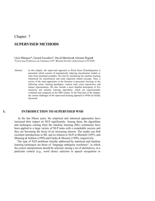
generalization bounds for the induced classifiers. The left plot in Figure 7-2
shows the geometrical intuition about the maximal margin hyperplane in a
two-dimensional space. The linear classifier is defined by two elements: a
weight vector w (with one component for each feature), and a bias b which
stands for the distance of the hyperplane to the origin. The classification rule
assigns +1 to a new example x, when f(x) = (x·w)+b > 0, and -1 otherwise.
The positive and negative examples closest to the (w,b) hyperplane (on the
dashed lines) are called support vectors.
Figure 7-2. Geometrical interpretation of Support Vector Machines
Learning the maximal margin hyperplane (w,b) can be simply stated as a
convex quadratic optimization problem with a unique solution, consisting of
(primal form): minimize ||w|| subject to the constraints (one for each training
example) yi [(w·xi) + b] ≥ 1, indicating that all training examples are
classified with a margin equal or greater than 1.
Sometimes, training examples are not linearly separable or, simply, it is
not desirable to obtain a perfect hyperplane. In these cases it is preferable to
allow some errors in the training set so as to maintain a better solution
hyperplane (see the right plot of Figure 7-2). This is achieved by a variant of
the optimization problem, referred to as soft margin, in which the
contribution to the objective function of the margin maximization and the
training errors can be balanced through the use of a parameter called C.
As seen in Section 2.4.6, SVMs can be used in conjunction with kernel
functions to produce non-linear classifiers. Thus, the selection of an
appropriate kernel to the dataset is another important element when using
SVMs. In the experiments presented below we used the SVMlight
software8
, a
freely available implementation. We have worked only with linear kernels,
performing a tuning of the C parameter directly on the DSO corpus. No
significant improvements were achieved by using polynomial kernels.
b/||w||
w
b/||w||
w

3.2 Empirical evaluation on the DSO corpus
We tested the algorithms on the DSO corpus. From the 191 words
represented in the DSO corpus, a group of 21 words which frequently appear
in the WSD literature was selected to perform the comparative experiment.
We chose 13 nouns (age, art, body, car, child, cost, head, interest, line,
point, state, thing, work) and 8 verbs (become, fall, grow, lose, set, speak,
strike, tell) and we treated them as independent classification problems. The
number of examples per word ranged from 202 to 1,482 with an average of
801.1 examples per word (840.6 for nouns and 737.0 for verbs). The level of
ambiguity is quite high in this corpus. The number of senses per word is
between 3 and 25, with an average of 10.1 senses per word (8.9 for nouns
and 12.1 for verbs).
Two kinds of information are used to perform disambiguation: local and
topical context. Let [w-3, w-2, w-1, w, w+1, w+2, w+3] be the context of
consecutive words around the word w to be disambiguated, and pi (-3 ≤ i ≤
3) be the part-of-speech tag of word wi. Fifteen feature patterns referring to
local context are considered: p-3, p-2, p-1, p+1, p+2, p+3, w-1, w+1, (w-2, w-1), (w-1,
w+1), (w+1, w+2), (w-3, w-2, w-1), (w-2, w-1, w+1), (w-1, w+1, w+2), and (w+1, w+2,
w+3). The last seven correspond to collocations of two and three consecutive
words. The topical context is formed by the bag-of-words {c1,...,cm}, which
stand for the unordered set of open class words appearing in the sentence.
The already described set of attributes contains those attributes used by
Ng (1996), with the exception of the morphology of the target word and the
verb-object syntactic relation. See Chapter 8 for a complete description of
the knowledge sources used by the supervised WSD systems to represent
examples.
The methods evaluated in this section codify the features in different
ways. AB and SVM algorithms require binary features. Therefore, local
context attributes have to be binarized in a pre-process, while the topical
context attributes remain as binary tests about the presence or absence of a
concrete word in the sentence. As a result of this binarization, the number of
features is expanded to several thousands (from 1,764 to 9,900 depending on
the particular word). DL has been applied also with the same example
representation as AB and SVM.
The binary representation of features is not appropriate for NB and kNN
algorithms. Therefore, the 15 local-context attributes are considered as is.
Regarding the binary topical-context attributes, the variants described by
Escudero et al. (2000b) are considered. For kNN, the topical information is
codified as a single set-valued attribute (containing all words appearing in
the sentence) and the calculation of closeness is modified so as to handle this
type of attribute. For NB, the topical context is conserved as binary features,

26 Chapter 7
but when classifying new examples only the information of words appearing
in the example (positive information) is taken into account.
3.2.1 Experiments
We performed a 10-fold cross-validation experiment in order to estimate
the performance of the systems. The accuracy figures reported below are
micro-averaged over the results of the 10 folds and over the results on each
of the 21 words. We have applied a paired Student’s t-test of significance
with a confidence value of t9,0.995=3.250see Dietterich (1998) for
information about statistical tests for comparing ML classification systems.
When classifying test examples, all methods are forced to output a unique
sense, resolving potential ties among senses by choosing the most frequent
sense among all those tied.
Table 7-2 presents the results (accuracy and standard deviation) of all
methods in the reference corpus. MFC stands for a most-frequent-sense
classifier, that is, a naive classifier that learns the most frequent sense of the
training set and uses it to classify all the examples of the test set. Averaged
results are presented for nouns, verbs, and overall and the best results are
printed in boldface.
Table 7-2. Accuracy and standard deviation of all learning methods
MFC NB kNN DL AB SVM
Nouns 46.59 ±1.08 62.29 ±1.25 63.17 ±0.84 61.79 ±0.95 66.00 ±1.47 66.80 ±1.18
Verbs 46.49 ±1.37 60.18 ±1.64 64.37 ±1.63 60.52 ±1.96 66.91 ±2.25 67.54 ±1.75
ALL 46.55 ±0.71 61.55 ±1.04 63.59 ±0.80 61.34 ±0.93 66.32 ±1.34 67.06 ±0.65
All methods clearly outperform the MFC baseline, obtaining accuracy
gains between 15 and 20.5 points. The best performing methods are SVM
and AB (SVM achieves a slightly better accuracy but this difference is not
statistically significant). On the other extreme, NB and DL are methods with
the lowest accuracy with no significant differences between them. The kNN
method is in the middle of the previous two groups. That is, according to the
paired t-test, the partial order between methods is:
SVM ≈ AB > kNN > NB ≈ DL > MFC
where ‘≈’ means that the accuracies of both methods are not significantly
different, and ‘>’ means that the left method accuracy is significantly better
than the right one.
The low performance of DL seems to contradict some previous research,
in which very good results were reported with this method. One possible
reason for this failure is the simple smoothing method applied. Yarowsky

(1995b) showed that smoothing techniques can help to obtain good estimates
for different feature types, which is crucial for methods like DL. These
techniques were also applied to different learning methods in (Agirre &
Martínez 2004b), showing a significant improvement over the simple
smoothing. Another reason for the low performance is that when DL is
forced to make decisions with few data points it does not make reliable
predictions. Rather than trying to force 100% coverage, the DL paradigm
seems to be more appropriate for obtaining high precision estimates. In
Martínez et al. (2002) DLs are shown to have a very high precision for low
coverage, achieving 94.90% accuracy at 9.66% coverage, and 92.79%
accuracy at 20.44% coverage. These experiments were performed on the
Senseval-2 datasets.
In this corpus subset, the average accuracy values achieved for nouns and
verbs are very close; the baseline MFC results are almost identical (46.59%
for nouns and 46.49% for verbs). This is quite different from the results
reported in many papers taking into account the whole set of 191 words of
the DSO corpus. For instance, differences of between 3 and 4 points can be
observed in favor of nouns in Escudero et al. (2000b). This is due to the
singularities of the subset of 13 nouns studied here, which are particularly
difficult. Note that in the whole DSO corpus the MFC over nouns (56.4%) is
fairly higher than in this subset (46.6%) and that an AdaBoost-based system
is able to achieve 70.8% on nouns (Escudero et al. 2000b) compared to the
66.0% in this section. Also, the average number of senses per noun is higher
than in the entire corpus. Despite this fact, a difference between two groups
of methods can be observed regarding the accuracy on nouns and verbs. On
the one hand, the worst performing methods (NB and DL) do better on
nouns than on verbs. On the other hand, the best performing methods (kNN,
AB, and SVM) are able to better learn the behavior of verb examples,
achieving an accuracy value around 1 point higher than for nouns.
Some researchers, Schapire (2002) for instance, argue that the AdaBoost
algorithm may perform poorly when training from small samples. In order to
verify this statement, we calculated the accuracy obtained by AB in several
groups of words sorted by increasing size of the training set. The size of a
training set is taken as the ratio between the number of examples and the
number of senses of that word, that is, the average number of examples per
sense. Table 7-3 shows the results obtained, including a comparison with the
SVM method. As expected, the accuracy of SVM is significantly higher than
that of AB for small training sets (up to 60 examples per sense). On the
contrary, AB outperforms SVM in the larger training sets (over 120
examples per sense). Recall that the overall accuracy is comparable in both
classifiers (Table 7-2).

28 Chapter 7
In absolute terms, the overall results of all methods can be considered
quite low (61-67%). We do not claim that these results cannot be improved
by using richer feature representations, by a more accurate tuning of the
systems, or by the addition of more training examples. Additionally, it is
known that the DSO words included in this study are among the most
polysemous English words and that WordNet is a very fine-grained sense
repository. Supposing that we had enough training examples for every
ambiguous word in the language, it seems reasonable to think that a much
more accurate all-words system could be constructed based on the current
supervised technology. However, this assumption is not met at present, and
the best current supervised systems for English all-words disambiguation
achieve accuracy figures around 65% (see Senseval-3 results). Our opinion
is that state-of-the art supervised systems still have to be qualitatively
improved in order to be really practical.
Table 7-3. Overall accuracy of AB and SVM classifiers by groups of words of increasing
average number of examples per sense
≤ 35 35-60 60-120 120-200 >200
AB 60.19% 57.40% 70.21% 65.23% 73.93%
SVM 63.59% 60.18% 70.15% 64.93% 72.90%
Apart from accuracy figures, the observation of the predictions made by
the classifiers provides interesting information about the comparison
between methods. Table 7-4 presents the percentage of agreement and the
Kappa statistic between all pairs of systems on the test sets. ‘DSO’ stands for
the annotation of the DSO corpus, which is taken as the correct annotation.
Therefore, the agreement rates with respect to DSO contain the accuracy
results previously reported. The Kappa statistic (Cohen 1960) is a measure
of inter-annotator agreement, which reduces the effect of chance agreement,
and which has been used for measuring inter-annotator agreement during the
construction of some semantically annotated corpora (Véronis 1998, Ng et
al. 1999b). A Kappa value of 1 indicates perfect agreement, values around
0.8 are considered to indicate very good agreement (Carletta 1996), and
negative values are interpreted as systematic disagreement on non-frequent
cases.
Table 7-4. Kappa statistic (below diagonal) and percentage of
agreement (above diagonal) between all pairs of systems on the DSO
corpus
DSO MFC NB kNN DL AB SVM
DSO — 46.6 61.5 63.6 61.3 66.3 67.1
MFC -0.19 — 73.9 58.9 64.9 54.9 57.3
NB 0.24 -0.09 — 75.2 76.7 71.4 76.7
kNN 0.39 -0.15 0.43 — 70.2 72.3 78.0

DSO MFC NB kNN DL AB SVM
DL 0.31 -0.13 0.39 0.40 — 69.9 72.5
AB 0.44 -0.17 0.37 0.50 0.42 — 80.3
SVM 0.44 -0.16 0.49 0.61 0.45 0.65 —
NB obtains the most similar results with regard to MFC in agreement rate
and Kappa value. The 73.9% of agreement means that almost 3 out of 4
times it predicts the most frequent sense (which is correct in less than half of
the cases). SVM and AB obtain the most similar results with regard to DSO
in agreement rate and Kappa values, and they have the less similar Kappa
and agreement values with regard to MFC. This indicates that SVM and AB
are the methods that best learn the behavior of the DSO examples. It is also
interesting to note that the three highest values of Kappa (0.65, 0.61, and
0.50) are between the top performing methods (SVM, AB, and kNN), and
that despite that NB and DL achieve a very similar accuracy on the corpus,
their predictions are quite different, since the Kappa value between them is
one of the lowest (0.39).
The Kappa values between the methods and the DSO annotation are very
low. But as Véronis (1998) suggests, evaluation measures should be
computed relative to the agreement between the human annotators of the
corpus and not to a theoretical 100%. It seems pointless to expect more
agreement between the system and the reference corpus than between the
annotators themselves. Besides, although hand-tagging initiatives that
proceed through discussion and arbitration report fairly high agreement rates
(Kilgarriff & Rosenszweig 2000), this is not the case when independent
groups hand-tag the same corpus separately. For instance, Ng et al. (1999b)
report an accuracy rate of 56.7% and a Kappa value of 0.317 when
comparing the annotation of a subset of the DSO corpus performed by two
independent research groups. Similarly, Véronis (1998) reports values of
Kappa near to zero when annotating some special words for the Romanseval
corpus9
(see Chapter 4).
From this point of view, the Kappa values of 0.44 achieved by SVM and
AB could be considered high results. Unfortunately, the subset of the DSO
corpus treated in this work does not coincide with Ng et al. (1999b) and,
therefore, a direct comparison is not possible.
4. CURRENT CHALLENGES OF THE SUPERVISED
APPROACH
Supervised methods for WSD based on machine learning techniques are
undeniably effective and they have obtained the best results up to date.

30 Chapter 7
However, there exists a set of practical questions that should be resolved
before stating that the supervised approach is a realistic way to construct
really accurate systems for wide-coverage WSD on open text. In this section,
we will discuss some of the problems and current efforts for overcoming
them.
4.1 Right-sized training sets
One question that arises concerning supervised WSD methods is the
quantity of data needed to train the systems. Ng (1997b) estimates that to
obtain a high accuracy domain-independent system, at least 3,200 words
should be tagged in about 1,000 occurrences per each. The necessary effort
for constructing such a training corpus is estimated to be 16 person-years,
according to the experience of the authors on the building of the DSO
corpus. However, Ng suggests that active learning methods, described
afterwards in this section, could reduce the required effort significantly.
Unfortunately, many people think that Ng’s estimate might fall short, as
the annotated corpus produced in this way is not guaranteed to enable high
accuracy WSD. In fact, recent studies using DSO have shown that: 1) The
performance for state of the art supervised WSD systems continues to be 60–
70% for this corpus (Escudero et al. 2001), and 2) Some highly polysemous
words get very low performance (20–40% accuracy).
There has been some work exploring the learning curves of each different
word to investigate the amount of training data required. Ng (1997b) trained
the exemplar-based-learning LEXAS system for a set of 137 words with at
least 500 examples each, and for a set of 43 words with at least 1,300
examples each. In both situations, the accuracy of the system was still rising
with the whole training data. In independent work, Agirre & Martínez (2000)
studied the learning curves of two small sets of words (containing nouns,
verbs, adjectives, and adverbs) using different corpora (SemCor and DSO).
Words of different types were selected, taking into account their
characteristics: high/low polysemy, high/low frequency, and high/low skew
of the most frequent sense in SemCor. Using decision lists as the learning
algorithm, SemCor is not big enough to get stable results. However, on the
DSO corpus, results seemed to stabilize for nouns and verbs before using all
the training material. The word set tested in DSO had on average 927
examples per noun, and 1,370 examples per verb.
The importance of having enough examples is also highlighted in our
experiment in Section 3.2.1., where the best performance is clearly achieved
on the set of words with more examples (more than 200 per sense).

4.2 Porting across corpora
The porting of the corpora to new genre/domains (cf. Chapter 10) also
presents important challenges. Some studies show that the assumptions for
supervised learning do not hold when using different corpora, and that there
is a dramatic degradation of performance.
Escudero et al. (2000c) studied the performance of some ML algorithms
(Naive Bayes, exemplar-based learning, decision lists, AdaBoost, etc.) when
tested on a different corpus (target corpus) than the one they were trained on
(source corpus), and explored their ability to adapt to new domains. They
carried out three experiments to test the portability of the algorithms. For the
first and second experiments, they collected two equal-size sets of sentence
examples from the WSJ and BC portions of the DSO corpus. The results
obtained when training and testing across corpora were disappointing for all
ML algorithms tested, since significant decreases in performance were
observed in all cases. In some of them the cross-corpus accuracy was even
lower than the most-frequent-sense baseline. A tuning technique consisting
of the addition of an increasing percentage of supervised training examples
from the target corpus was applied. However, this did not help much to raise
the accuracy of the systems. Moreover, the results achieved in this mixed
training situation were only slightly better than training on the small
supervised part of the target corpus, making no use at all of the set of
examples from the source corpus.
The third experiment showed that WSJ and BC have very different sense
distributions and that relevant features acquired by the ML algorithms are
not portable across corpora, since they were indicating different senses in
many cases.
Martínez & Agirre (2000) also attribute the low performance in cross-
corpora tagging to the change in domain and genre. Again, they used the
DSO corpus and a disjoint selection of the sentences from the WSJ and BC
parts. In BC, texts are classified according to predefined categories
(reportage, religion, science-fiction, etc.); this allowed them to perform tests
on the effect of the domain and genre on cross-corpora tagging.
Their experiments, training on WSJ and testing on BC and vice versa,
show that the performance drops significantly from the performance on each
corpus separately. This happened mainly because there were few common
collocations, but also because some collocations received systematically
different tags in each corpus—a similar observation to that of Escudero et al.
(2000c). Subsequent experiments were conducted taking into account the
category of the documents of the BC, showing that results were better when
two independent corpora shared genre/topic than when using the same
corpus with different genre/topic. The main conclusion is that the one sense

32 Chapter 7
per collocation constraint does hold across corpora, but that collocations
vary from one corpus to other, following genre and topic variations. They
argued that a system trained on a specific genre/topic would have difficulties
to adapt to new genres/topics. Besides, methods that try to extend
automatically the set of examples for training should also take into account
these phenomena.
4.3 The knowledge acquisition bottleneck
As we mentioned in the introduction, an important issue for supervised
WSD systems is the knowledge acquisition bottleneck. In most of the
tagged corpora available it is difficult to find at least the required minimum
number of occurrences per each sense of a word. In order to overcome this
problem, a number of lines of research are currently being pursued,
including: (i) Automatic acquisition of training examples; (ii) Active
learning; (iii) Combining training examples from different words; (iv)
Exploiting parallel corpora; and (v) Learning from labeled and unlabeled
examples. We will focus on the former four in this section, and devote the
next section to the latter.
In automatic acquisition of training examples (see Chapter 9), an
external lexical source, for instance WordNet, or a sense-tagged corpus is
used to obtain new examples from a very large untagged corpus (e.g., the
Internet).
Leacock et al. (1998) used a pioneering knowledge-based technique to
automatically find training examples from a very large corpus. WordNet was
used to locate monosemous words semantically related to those word senses
to be disambiguated (monosemous relatives). The particular algorithm is
described in Chapter 9.
In a similar approach, Mihalcea & Moldovan (1999) used information in
WordNet (e.g., monosemous synonyms and glosses) to construct queries,
which later fed the Altavista10
web search engine. Four procedures were used
sequentially, in a decreasing order of precision, but with increasing levels of
retrieved examples. Results were evaluated by hand finding out that over
91% of the examples were correctly retrieved among a set of 1,080 instances
of 120 word senses. However, the number of examples acquired does not
have to correlate with the frequency of senses, and the resulting corpus was
not used for training a real WSD system.
Mihalcea (2002a) generated a sense tagged corpus (GenCor) by using a
set of seeds consisting of sense-tagged examples from four sources: SemCor,
WordNet, examples created using the method above, and hand-tagged
examples from other sources (e.g., the Senseval-2 corpus). A corpus with
about 160,000 examples was generated from these seeds. A comparison of

the results obtained by the WSD system, when training with the generated
corpus or with the hand-tagged data provided in Senseval-2, was reported.
She concluded that the precision achieved using the generated corpus is
comparable, and sometimes better, than learning from hand-tagged
examples. She also showed that the addition of both corpora further
improved the results in the all-words task. Their method has been tested in
the Senseval-2 framework with good results for some words.
This approach was also taken by Agirre and Martinez (2004c), where they
rely on monosemous relatives of the target word to query the Internet and
gather sense-tagged examples. In this case, they analyze the effect of the bias
of the word senses in the performance of the system. They propose to
integrate the work from McCarthy et al. (2004), who devised a method to
automatically find the predominant senses in an unlabeled corpus. Although
this latter study only solves partially the problem, and is limited to nouns
only, it seems to be very promising (see Chapter 6 for details). Combining
this method with their automatically sense-tagged corpus, Agirre and
Martinez (2004c) improve over the performance of the best unsupervised
systems in English Senseval-2 lexical-sample.
Following also similar ideas, Cuadros et al. (2004) present ExRetriever, a
software tool for automatically acquiring large sets of sense tagged examples
from large collections of text or the Web. This tool has been used to directly
compare on SemCor different types of query construction strategies. Using
the powerful and flexible declarative language of ExRetriever, new
strategies can be easily designed, executed and evaluated.
Active learning is used to choose informative examples for hand-
tagging, in order to reduce the acquisition cost. Argamon-Engelson & Dagan
(1999) describe two main types of active learning: membership queries and
selective sampling. In the first approach, the learner constructs examples and
asks a teacher to label them. This approach would be difficult to apply to
WSD. Instead, in selective sampling the learner selects the most informative
examples from unlabeled data. The informativeness of the examples can be
measured using the amount of uncertainty in their classification, given the
current training data. Lewis & Gale (1994) use a single learning model and
select those examples for which the classifier is most uncertain (uncertainty
sampling). Argamon-Engelson & Dagan (1999) propose another method,
called committee-based sampling, which randomly derives several
classification models from the training set, and the degree of disagreement
among them is used to measure the informativeness of the examples.
Regarding WSD, Fujii et al. (1998) applied selective sampling to the
acquisition of examples for disambiguating verb senses, in an iterative
process with human taggers. The disambiguation method was based on

34 Chapter 7
nearest neighbor classification, and the selection of examples via the notion
of training utility. This utility is determined based on two criteria: Number
of neighbors in unsupervised data (i.e., examples with many neighbors will
be more informative in next iterations), and similarity of the example with
other supervised examples (the less similar, the more interesting). A
comparison of their method with uncertainty and committee-based sampling
showed a significantly better learning curve for the “training utility”
approach.
Open Mind Word Expert (Chklovski & Mihalcea 2002) is a project to
collect sense-tagged examples from web users (see Section 2.1 in this
chapter, and also Section 3.4 of Chapter 9). They select the examples to be
tagged applying a selective sampling method. Two different classifiers are
independently applied on untagged data: an instance-based classifier that
uses active feature selection, and a constraint-based tagger. Both systems
have a low inter-annotation agreement, high accuracy when they agree, and
low accuracy when they disagree. This makes the disagreement cases the
hardest to annotate, therefore they are presented to the user.
Another recent trend to alleviate the knowledge acquisition bottleneck is
the combination of training data from different words. In (Kohomban
and Lee, 2005) they build semantic classifiers by merging the training data
from words in the same semantic class. Once the system selects the class,
simple heuristics are applied to obtain the fine-grained sense. The classifier
follows the memory-based learning paradigm, and the examples are
weighted according to their semantic similarity to the target word (computed
using WordNet similarity). Their final system improved the overall results of
the Senseval-3 all-words competition. Another approach that uses training
data from different words in their model is presented in (Niu et al., 2005).
They build a word-independent model to compute the similarity between
two contexts. A maximum entropy algorithm is trained with the all-words
Semcor corpus, and the model is used for clustering the instances of a given
target word. One usual problem of clustering systems is the evaluation, and
in this case they map the clusters to the Senseval-3 lexical-sample data by
looking at 10% of the examples in the training data. Their final system
obtained the best results for unsupervised systems on the English Senseval-3
lexical-sample task.
Another potential source for automatically obtaining WSD training data
is parallel corpora. This approach was already suggested a few years ago
by Resnik & Yarowsky (1997) but only recently has been applied to real
WSD. The key point is that by using the alignment tools from the Statistical
Machine Translation community one can unsupervisedly align at word level
all the sentence pairs in both languages. By using the alignments in the two
directions and some knowledge sources (e.g., WordNet) to test consistency

and eliminate noisy alignments, one can extract all possible translations for
each given word in the source language, which, in turn, can be considered as
the relevant senses to disambiguate. Two recent papers present very
promising evidence for the validity of this approach (Chan & Ng 2005, Tufis
et al. 2005). The former validates the approach by evaluating on the
Senseval-2 all-words setting (restricted to nouns), which implies to map the
coarse-grained senses coming from translation pairs to the fine-grained sense
inventory of WordNet. They conclude that using a Chinese-English parallel
corpus of 680MB is enough to achieve the accuracy of the best Senseval-2
system at competition time.
4.4 Bootstrapping
As a way to partly overcome the knowledge acquisition bottleneck, some
methods have been devised for building sense classifiers when only a few
annotated examples are available jointly with a high quantity of unannotated
examples. These methods, which use labeled and unlabeled data are also
referred to as bootstrapping methods (Abney 2002; 2004). Among them,
we can highlight co-training (Blum & Mitchell 1998), their derivatives
(Collins & Singer 1999; Abney 2002, 2004), and self-training (Nigam &
Ghani 2000).
In short, co-training algorithms work by learning two complementary
classifiers for the classification task trained on a small starting set of labeled
examples, which are then used to annotate new unlabeled examples. From
these new examples, only the most confident predictions are added to the set
of labeled examples, and the process starts again with the re-training of
classifiers and re-labeling of examples. This process may continue for
several iterations until convergence, alternating at each iteration from one
classifier to the other. The two complementary classifiers are constructed by
considering two different views of the data (i.e., two different feature
codifications), which must be conditionally independent given the class
label. In several NLP tasks, co-training generally provided moderate
improvements with respect to not using additional unlabeled examples.
One important aspect of co-training consist on the use of different views
to train different classifiers during the iterative process. While Blum &
Mitchell (1998) stated the conditional independence of the views as a
requirement, Abney (2002) shows that this requirement can be relaxed.
Moreover, Clark et al. (2003) show that simply re-training on all the newly
labeled data can, in some cases, yield comparable results to agreement-based
co-training, with only a fraction of the computational cost.
Self-training starts with a set of labeled data, and builds a unique
classifier (there are no different views of the data), which is then used on the

36 Chapter 7
unlabeled data. Only those examples with a confidence score over a certain
threshold are included to the labeled set. The classifier is then retrained on
the new set of labeled examples. This process continues for several
iterations. Notice that only a single classifier is derived. The Yarowsky
algorithm, already described in Section 2.4.6 (Yarowsky 1995a) and
theoretically studied by Abney (2004), is the best known representative of
this family of algorithms. These techniques seem to be appropriate for WSD
and other NLP tasks because of the wide availability of raw data and the
scarcity of annotated data.
Mihalcea (2004) introduces a new bootstrapping schema that combines
co-training with majority voting, with the effect of smoothing the
bootstrapping learning curves, and improving the average performance.
However, this approach assumes a comparable distribution of classes
between both labeled and unlabeled data (see section 4.2). At each iteration,
the class distribution in the labeled data is maintained, by keeping a constant
ratio across classes between already labeled examples and newly added
examples. This implies to know a priori the distribution of sense classes in
the unlabeled corpus, which seems unrealistic. Maybe, a possible solution to
this cycling problem will come from the work of McCarthy et al. (2004),
introduced in section 4.3.
Pham et al. (2005) also experimented with a number of co-training
variants on the Senseval-2 WSD lexical sample and all-words settings,
including the ones presented in Mihalcea (2004). Although the original co-
training algorithm did not provide any advantage over using only labeled
examples, all the sophisticated co-training variants obtained significant
improvements (taking Naive Bayes as the base learning method). The best
method reported was Spectral-Graph-Transduction Cotraining.
4.5 Feature selection and parameter optimization
Another current trend in WSD is the automatic selection of features.
Some recent work has focused on defining separate feature sets for each
word, claiming that different features help to disambiguate different words.
The exemplar-based learning algorithm is very sensitive to irrelevant
features, so in order to overcome this problem Mihalcea (2002b) used a
forward-selection iterative process to select the optimal features for each
word. She ran cross-validation on the training set, adding the best feature to
the optimal set at each iteration, until no improvement was observed. The
final system achieved good results in the Senseval-2 competition.
Very interesting research has been conducted connecting parameter
optimization and feature selection for WSD. Hoste et al. (2002b) observed
that although there have been many comparisons among ML algorithms

trying to determine the method with the best bias for WSD, there are large
variations on performance depending on three factors: algorithm parameters,
input representation (i.e., features), and interaction between both. They claim
that changing any of these factors produces large fluctuations in accuracy,
and that exhaustive optimization of parameters is required in order to obtain
reliable results. They argue that there is little understanding of the interaction
among the three influential factors, and while no fundamental data-
independent explanation is found, data-dependent cross-validation can
provide useful clues for WSD. In their experiments, they show that memory-
based WSD benefits from optimizing architecture, information sources, and
algorithmic parameters. The optimization is carried out using cross-
validation on the learning data for each word. In order to do it, one
promising direction is the use of genetic algorithms (Daelemans & Hoste
2002), which lead to very good results in the Senseval-3 English all-words
task (Decadt et al. 2004)—though the results were less satisfactory in the
English lexical-sample task.
Martínez et al. (2002) made use of feature selection for high precision
disambiguation at the cost of coverage. By using cross validation on the
training corpus, a set of individual features with a discriminative power
above a certain threshold was extracted for each word. The threshold
parameter allows to adjust the desired precision of the final system. This
method was used to train decision lists, obtaining 86% precision for 26%
coverage, or 95% precision for 8% coverage on the Senseval-2 data. In
principle, such a high precision system could be used to acquire almost
error-free new examples in a bootstrapping framework.
Another approach to feature engineering consists in using smoothing
methods to optimize the parameters of the models. In (Agirre and Martinez,
2004c), they integrate different smoothing techniques from the literature
with four well-known ML methods. The smoothing techniques focus on the
different feature types and provide better probability estimations for dealing
with sparse data. They claim that the systems are more robust when
integrating smoothing techniques. They combine the single methods and
their final ensemble of algorithms improves the best results in the English
Senseval-2 lexical-sample task.
4.6 Combination of algorithms and knowledge sources
The combination paradigm, known as ensembles of classifiers, is a very
well-known approach in the machine learning community. It helps to reduce
variance and to provide more robust predictions for unstable base classifiers.
The key for improving classification results is that the different classifiers
combined commit non-correlated errors. For an in-depth analysis on

Supervised Corpus-based Methods for Word Sense Disambiguation

Supervised Corpus-based Methods for Word Sense Disambiguation

Recommandé

Recommandé

Contenu connexe

Tendances

Tendances (18)

Similaire à Supervised Corpus-based Methods for Word Sense Disambiguation

Similaire à Supervised Corpus-based Methods for Word Sense Disambiguation (20)

Plus de butest

Plus de butest (20)

Supervised Corpus-based Methods for Word Sense Disambiguation