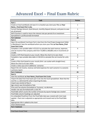
1. Advanced Excel – Final Exam Rubric
Task Points
Part 1
Create an Excel workbook and save it in a location you store your files as Your 1
Name_ Final Exam Part 1.xlsx
Current Savings Amount, Goal Amount, monthly Deposit Amount, and years to save 1
are all present
RATE function is used to return the interest rate per period of an investment 6
Spreadsheet is professionally formatted 2
Part Subtotal 10
Part 2:
Open the workbook Final Exam Part 2.xlsx from the Final Project Assignment folder 1
in Blackboard. Save the workbook where you store your files as Your Name_Final
Exam Part 2.xlsx
Complete a one-variable table in E5:G11 to calculate the total revenue, expenses, 4
and net income if the company sells from 75,000 to 200,000 units in increments of
25,000.
Create a CVP Chart based on your results. Move the chart to its own sheet. 4
Complete a two-variable data table in E18:I24 to calculate the net income for units 4
sold
Create a Plot chart based on your results (Hint: use scatter with straight lines). 4
Move the chart to its own sheet.
Create a status quo and 3 additional scenarios 4
Report the net income, revenue and total expenses for each scenario in a scenario 4
summary report.
Part 2 Subtotal 25
Part 3:
Save the workbook as Your Name_Final Exam Part 3.xlsx 1
Import the data from final exam part 3.txt into the Excel spreadsheet. Note that the 3
text file is a delimited file when importing the data.
Import was started at Row 5. 3
Age column was formatted as Text. 2
Price and Tax columns formatted as ‘Currency’, no decimals 2
Header row was formatted with a color fill. 2
PivotTable which counts the number of houses by square footage was created 4
PivotTable column headings are adjusted 1
An embedded PivotChart from the PivotTable data was created with chart style 4
applied. Chart size is adjusted as appropriate and moved next to the PivotTable
data.
Appropriate title is added to the chart 1
Chart Sheetsnamed. 2
Part 3 Subtotal: 25
Final Exam Grand Total 60