Breaking the Kubernetes Kill Chain: Host Path Mount
GPS and Digital Terrain Elevation Data (DTED) Integration
1. GPS and Digital Terrain Elevation Data (DTED)
Integration
M. Phatak, G. Cox, L. Garin, SiRF Technology Inc.
(DTM). These models are available from various
BIOGRAPHIES
government agencies and depending on the application,
DTMs have relatively accurate vertical elevations
Makarand Phatak is currently Staff Systems Engineer at
sufficient enough to be used for aiding GPS constrained
SiRF Technology Inc. where he has been for over three
heights for E-911 or LBS. For the purpose of this study
years. Prior to joining SiRF he worked at Siemens for two
the National Imagery and Mapping Agency (NIMA)
years on pattern recognition applied primarily to speaker
Digital Terrain Elevation Data (DTED®) Level 0 was
pattern recognition identification and Aerospace Systems
used. To integrate DTM data in LSQ constrained height
for five years on design of GPS navigation algorithms
conditions a fourth order polynomial equation is formed.
such as GPS and GPS/INS integrated Kalman filters and
Results from integrating DTM data into the LSQ
fault detection and identification. He holds a Ph. D.
navigation algorithm is very promising.
degree in control systems from the Indian Institute of
Science, Bangalore, India and M. Tech. in electrical
engineering from the Indian Institute of Technology,
Kharagpur, India. INTRODUCTION
Geoffrey F. Cox is currently Staff Engineer at SiRF GPS weak signal acquisition and tracking with the use of
Technology, Inc. where he as been since 2000. Before high sensitivity autonomous or network centric GPS
joining, SiRF Mr. Cox worked in various areas of GPS receivers in urban and rural indoor or outdoor
application development for Satloc, Inc., Nikon, Inc., and environments will allow for navigation in these
NovAtel, Inc. from 1996 to 2000. He holds M. Eng. in environments, MacGougan, G. et. al. (2002) and Garin, L.
Geomatics Engineering from the University of Calgary. et. al. (1999). However, strong signal shading and fading
effects compounds a GPS receiver’s ability to acquire and
Lionel J. Garin, Director of Systems Architecture and
track SVs and if the effects are strong enough the
Technology, SiRF Technology Inc., has over 20 years of
resulting navigation using a minimum number of 3 SVs
experience in GPS and communications fields. Prior to
for 2D or 4 SVs for 3D navigation can have negative
that, he worked at Ashtech, SAGEM and Dassault
impacts of desired horizontal accuracy. Accurate 2D
Electronique. He is the inventor of the quot;Enhanced Strobe
navigation is further impacted if the GPS receiver handset
Correlatorquot; code and carrier multipath mitigation
device is used in a high elevation urban/suburban
technology. He holds an MSEE equivalent degree in
environment for example, Denver, CO, USA or Calgary,
digital communications sciences and systems control
Alberta, CAN. Typical application scenarios for 2D GPS
theory from Ecole Nationale Superieure des
navigation is to use some type of externally provided
Telecommunications, France and BS in physics from
height and its uncertainty. Such methods are: last known
Paris VI University.
calculated height (stored in receiver memory from
previous 3D navigation), network provided height
through cell location or Base Station (BS) as well as
ABSTRACT through the use DTM models, Moeglein, M. and N.
Krasner (1998) and external sensors, Stephen, J., and G.
The use of GPS for personal location using cellular
Lachapelle (2001).
telephones or personal handheld devices requires signal
measurements in both outdoor and indoor environments
for E-911 and Location Based Services (LBS). Therefore,
DIGITAL TERRIAN ELEVATION DATA (DTED®)
minimal satellite (SV) measurements such as a 3 SV or 4
DESCRIPTION
SV acquisition, tracking and navigation fix in many
situations will be encountered. To overcome 2D
In 1999, the NIMA released a standard digital dataset
navigation side effects, such as increased horizontal
DTED® Level 0 for the purpose of commercial and
uncertainty and error, because of constraining an
public use. This DTED® product provides a world wide
inaccurately obtained height in Least Squares (LSQ) can
coverage and is a uniform matrix of terrain elevation
be minimized using an integrated Digital Terrain Model
2. values which provides basic quantitative data for systems EARTH GRAVITY MODEL (EGM) DESCRIPTION
and applications that require terrain elevation, slope,
and/or surface roughness information. DTED® Level 0 GPS is referenced to the WGS-84 ellipsoid and the
elevation post spacing is 30 arc second (nominally one computed navigation heights are either, above/below
kilometer). In addition to this discrete elevation file, ellipsoid ( h ). It is desired to aid the constrained height
separate binary files provide the minimum, maximum, through the means of Orthometric ( H ) to h conversion.
and mean elevation values computed in 30 arc second To do this, the EGM is employed to obtain h from the
square areas (organized by one degree cell). DTED® H . For the purpose of this paper, the EGM
(1984) was used. Currently there is an EGM (1996)
The DTED® Level 0 contains the NIMA Digital Mean
available for use from NIMA and arguably would not
Elevation Data (DMED) providing minimum, maximum,
improve on reducing absolute LE errors associated with
and mean elevation values and standard deviation for each
using the DTED® Level 0 unless a more accurate
15 minute by 15 minute area in a one degree cell. This
DTED® Level is used or other sourced DTM.
initial prototype release is a quot;thinnedquot; data file extracted
from the NIMA DTED® Level 1 holdings where
available and from the elevation layer of NIMA VMAP Table 2 EGM - 84
Level 0 to complete near world wide coverage. The
Horizontal DATUM WGS-84
specifications for DTED® Level 0 are:
Coverage World Wide
10o by 10o
Grid Spacing
Table 1 DTED® Performance Specification (1996) Relative Vert. Accuracy 3 (m) LE
Horizontal DATUM WGS-84
ALGORITHM OUTLINE
Coverage World Wide
1o by 1o First, the idea is to form a fourth equation from the
Tile (Individual File)
DTED®. This equation is derived from a polynomial (in
Coverage
2 variables of northing φ and easting λ ) surface fit to
Grid Spacing ~1 Km (30’)
the appropriate terrain. To select this appropriate terrain
Absolute Hor. Accuracy 90% Circular Error (CE) the 3 SV measurements are solved first for a fixed h .
≤ 50 (m)
The fixed h is the average value of the h in the
neighborhood of the BS (Base Station). Typically, the
Absolute Vert. Accuracy 90% Linear Error (LE)
boundary of this neighborhood is a few tens of kilometers
≤ 30 (m)
away from the BS (as the center). Error in the fixed h is
90% CE WGS ≤ 30 (m)
Relative Hor. Accuracy
taken as the standard deviation of h in the neighborhood.
over a 1o cell
(point to point)
With this information the 3 SV position solution with
90% CE WGS ≤ 20 (m)
Relative Vert. Accuracy fixed altitude comes with an estimated error ellipse.
over a 1o cell
(point to point)
Secondly, it is required to construct grid points along the
directions of the major and minor axes of the error ellipse.
The step sizes are made proportional to the magnitudes of
One technical issue to point out is the NIMA still reserved
the major and minor axes respectively. The center of the
the right to not include sensitive military installations here
ellipse is the 3 SV position as obtained before. Along the
in the US and abroad. Those areas deemed sensitive do
semi-major axis 9 points are selected (4 in the positive
not include elevation data but rather horizontal positions
direction, 4 in the negative and one at the center) and
and will appear delineated as an empty space if using a
along the semi-major axis 5 points are selected (2 in the
mapping package to visualize the terrain. Therefore, if an
positive direction, 2 in the negative and one at the center)
E-911 or LBS system requires seamless DTM coverage
to cover a rectangular grid of 4 sigma along each axis. In
there are other models available with similar performance
this process, 45 points are chosen in the rectangular grid.
specifications, namely GTOPO30 Global Elevation
Altitude values above the mean sea level ( H ) at these
Model, GTOPO30 Documentation (1996).
points are obtained from the DTED® by indexing the four
corner points in which the grid point resides and then
GTOPO30 is a global digital elevation model (DEM) with
using bilinear interpolation between these corner points.
a horizontal grid spacing of 30 arc seconds
The obtained H values are converted to the WGS 84 h
(approximately 1 kilometer). The DEM was derived from
several raster and vector sources of topographic by adding the Geoid N separation at the 3 SV position
information. The coverage and accuracy specification are point.
similar to that of the DTED® Level 0.
3. φ , λ and h as well as a 4) Fit a 2-D polynomial of degree 4 in the variables
Thirdly, the grid of 45 points of
of φ and λ with a total of 15 coefficients to the
φ and λ is found using LSQ
4-th order polynomial in
45 points obtained in step 3. Find the maximum
method. There are 15 coefficients to determine. To
residual error for the polynomial fit. If this error
handle ill conditioning the polynomial is found in new
exceeds a threshold of 100 m stop processing
variables that represent a scaled deviation from the center
with appropriate error message, else proceed
point (the 3 SV position solution). Also a robust
along to step five.
numerical method of Q-R decomposition is used; with Q
computed using modified Gram-Schmidt procedure (to
5) Solve GPS equations with 3 SV pseudorange
make Q only orthogonal rather than orthonormal); this is
measurements and the equation of the
to avoid square root operations. The equation of the
polynomial along with the maximum residual
polynomial with so determined coefficients is the 4-th
error of step 4 to find position and horizontal
equation. The maximum deviation of the grid point
error ellipse parameters.
altitude from the surface fit is the error associated with
this 4-th equation. If this error exceeds a given threshold
6) For the φ and λ as obtained in step 5 check
(empirically derived and set to 100 meters) then the
polynomial fit is declared poor and unusable. Then more whether the corresponding point belongs to the
than one polynomial surface fits are required. rectangular grid of step 3 and if yes accept the
solution of step 5 as a valid solution else reject it
Lastly, the 3 GPS equations and the 4-th polynomial
as invalid.
equation are solved in coordinates of φ , λ , h and clock
bias rather than using Earth Center Earth Fixed (ECEF).
COMPLETE EQUATIONS
The ECEF coordinate formulation is retained and change
from ECEF to chosen coordinates is achieved by working
DTED® Level 0 Indexing
with the corresponding Jacobian. The Jacobian
corresponding to the 4-th equation comes from the
φu λu , the nearest
Given a user latitude, and longitude,
derivative of the polynomial. If there is a convergence
then it is checked whether the converged solution is South-West corner of an available DTED® data file is
within the rectangular grid of polynomial fit. If it is not found and used as a reference to find an index in that data
then the method is repeated for the next surface fit if file. This index is used to retrieve the H . The equations
available. are found on the next page.
y = λu − λr
[1]
Algorithm In Steps
where,
1) With the reference location at the center retrieve
Orthometric heights at points 1 km apart in the
λr Reference Longitude for the South West Corner
Easting and Northing directions. A total of
of an available DTED data file.
(2 ⋅ N + 1) 2 points are considered on a grid of
λu Apriori/User Longitude.
(2 ⋅ N + 1) × (2 ⋅ N + 1) points. Convert the
y Difference in degrees
Orthometric H to WGS 84 h . Determine
average h and set h error equal to the standard
x = φu − φ r
[2]
deviation over the grid of points..
2) Solve GPS equations with 3 SV pseudorange where,
measurements and average h and the h error in
φr
step 1 to find the position and corresponding Reference Latitude for the South West Corner of
horizontal error ellipse parameters.
an available DTED data file.
φu User Latitude.
3) With the position of step 2 at the center, retrieve
H at points on a rectangular grid constructed x Difference in degrees .
along the major and minor axes of the ellipse. A
total of 45 points are considered on a grid of
y ∗ 3600
9 × 5 points. [3] brow =
∆ λ spacing
4. (φ u − φ 3 )3600
[5] x' =
(∆ φ )
where, − bcol
spacing
where,
∆λspacing DTED Level 0 Grid Spacing of 30” Arc
Seconds x' Weighted Ratio from user/reference Latitude
brow Integer Row value within DTED data grid spacing and DTED column location.
file in the range [0, 129].
(λ u − λ 3 )3600
y' =
[6]
(∆ λ − brow )
x * 3600 spacing
[4] bcol = where,
∆ φ spacing
y ' Weighted Ratio from user/reference Longitude
where,
grid spacing and DTED column location.
∆φspacing DTED Level 0 Grid Spacing of
[7]
30” Arc Seconds
H i = H1 + (H 2 − H1 )x'+(H 4 − H1 ) y'+(H1 + H 3 − H 2 − H 4 )x' y'
bcol Integer Column value within
DTED data file in the range [0,
129]. where,
The values of brow and bcol are used to find the index in H 1 , L , H 4 , represent 4 Orthometric heights in a given
the data file and then this index is used to access the
searched row and column result.
altitude value.
H i is the interpolated Orthometric height and 45 of these
points are determined.
1× 1Deg.
y'
Height above Ellipsoid Estimation
H3 H4
To estimate the 45 points of h requires the estimation of
H 3, 4
x'
the Geoid N from the EGM-84 as a function of φu and
Hi
λu .
H1, 2
H1
Row
H2
Once N is estimated a linear calculation is used to
determine h , Schwarz, K, and Krynski, J. (1994). Figure
(φ r , λr )
2 below illustrates the relationship for computing between
Col
the DTED® model and EGM-84 model.
SW Corner Reference
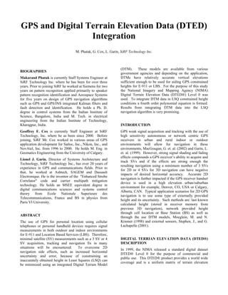
Figure 1: Indexing and Bilinear Interpolation Scheme
h=N+H
[8]
Bilinear Interpolation pt25
The H is obtained as above and interpolated to the given pt1
user latitude, φu and longitude, λu as follows. The brow Topography
H 25
H1 h25
h1
φ3
Geoid Model
and bcol correspond to the altitude H 3 , latitude, and True Geoid
N 25
N1
λ3 ;
longitude, see figure 1. Three more altitudes H 1 , Ellipsoid
(WGS-84)
and H 4 are obtained from (brow+1) and bcol,
H2
(brow+1) and (bcol+1) and brow and (bcol+1)
Figure 2: Vertical Relationships
respectively. Then, H , at φu and λu is obtained as
Constrained LSQ Solution from 3 SV Pseudoranges
follows:
and Average h
The equations to be solved are:
5. [9] approximation using Taylor series gives the following
equations.
( s1x − px ) 2 + ( s1 y − p y ) 2 + ( s1z − pz ) 2 ⋅ (1 − m1 ) + b = ρ1
− l1x − l1 y − l1z 1 ∆px ∆ρ1
( s2 x − px ) 2 + ( s2 y − p y ) 2 + ( s2 z − pz ) 2 ⋅ (1 − m2 ) + b = ρ 2
− l 1 ∆p y ∆ρ 2
− l2 y − l2 z
2x ⋅
( s3 x − px ) 2 + ( s3 y − p y ) 2 + ( s3 z − pz ) 2 ⋅ (1 − m3 ) + b = ρ3 = ,
[11]
− l3 x 1 ∆pz ∆ρ3
− l3 y − l3 z
( p 'x − px ) 2 + ( p ' y − p y ) 2 + ( p'z − pz ) 2 ⋅ sgn(h) = h
− d x − dy − dz 0 ∆b ∆h
where ( s ix , s iy , s iz ) are the ECEF coordinates of antenna
phase center of SV i at the receive time, ( p x , p y , p z ) where, l i is line of sight unit vector pointing from
are the ECEF coordinates of the GPS receiver antenna receiver to SV i and d is down direction unit vector
phase center, b is common offset in pseudorange pointing along the downward normal to the WGS-84
measurements, ρ i is i -th pseudorange measurement, ellipsoid, ∆p x , ∆p y , and ∆p z are differential position
coordinates, ∆b is differential pseudorange offset, ∆ρ1 ,
mi satellite mean motion correction term (given below),
∆ρ 2 , and ∆ρ 3 are differential pseudoranges, and ∆h is
( p' x , p' y , p' z ) are ECEF coordinates of projection of
( p x , p y , p z ) on the WGS-84 ellipsoid, ρ i is the differential h . The line of sight unit vector is given by
measured pseudorange for SV i , h is the height above
WGS-84 ellipsoid and sgn( h) = 1 if h > 0 , [12]
sgn(h) = −1 if h < 0 , and it is undefined when h = 0
(here the equation itself reduces to an identity but the
,
1
differential version of the equation is still defined; see li = ⋅ (si − p * )
( s ix − p * ) 2 + ( s iy − p * ) 2 + ( s iz − p * ) 2
below). The h is given by the average h as obtained x y z
from the step 1 of the above algorithm. The receive time
is assumed to be have error less than about 10 ms so that
the satellite positions as computed from the ephemeris the down direction unit vector is given by
have good accuracy. The mean motion correction term,
mi is given as
− cos λ* ⋅ cos φ *
d = − sin λ* ⋅ cos φ * ,
[13]
1
mi = ⋅ (vi + ω × s i ) o (si − p ),
− sin φ *
[10]
c
where × denotes vector cross product, o denotes vector
(φ * , λ* , h * ) are the WGS-84 geodetic
where
dot product, vi is the velocity vector of SV i , s i is the
*
coordinates of p (the equations for change of
position vector of SV i , ω is the Earth rotation vector
coordinates are not included in this document, Kaplan, D.
and p is GPS receiver position vector, the x , y , and
(1996)),
z coordinates of all vectors are in ECEF and all except
ω correspond to the antenna phase centers.
∆ρ i = ρ i − ρ i* ,
[14]
* * *
Let ( p , p , p ) be the ECEF coordinates of the
x y z
ρ i*
where are obtained from the left hand side of [9] at
reference or approximate position which serves as the
the initial guess point, and
*
initial guess for ( p x , p y , p z ) and let b be the initial
guess for the pseudo-range offset. Expanding the left hand
side of [10] around the initial guess to a first order
∆h = h − h * .
[15]
6. m(n) = m(n − 1) + (n + 1) with m(0) = 1.
Equation [11] is solved for ∆p x , ∆p y , ∆p z and ∆b . For
degree, n = 4 , m = 15 . The coefficients, ci ,
Then the estimates of position and clock bias are updated
as
i = 1,L, m are obtained by solving the following linear
equation [20] using least squares method.
p x p * ∆p x
ˆ [20]
x
p * ∆p
ˆy c0
py y
= +
[16] . c
p z p * ∆p z
ˆ 1
z
ˆ * c2 ξ1
φ1 λ1 φ12 φ1 ⋅ λ1 λ12 L λ1n 1
b b ∆b
1 c3 ξ 2
φ2 λ2 φ2 φ2 ⋅ λ2 λ2 L λ2n
2 2
=
⋅
M c4 M
M M M M M OM
This is the Newton-Raphson update. Next, the initial
1 M ξ r
φr λr φr φr ⋅ λr λr L λrn
2 2
guess is replaced by the new estimate as
cm−2
cm−1
p* px
ˆ
x
* ˆ where the subscript i (except on the coefficient)
py = py ,
[17] represents i -th point of the terrain. The points are chosen
p* pz
ˆ
as follows. The center point (as given by φ c , λc , and
z
* ˆ
b b
ξc ) is the point which corresponds to the solution
obtained in step 2. This solution also comes with
horizontal error ellipse parameters of the semi-major axis,
and the iterations are continued until ∆p x , ∆p y , ∆p z
a e , the semi-minor axis, be , and the angle the semi-
and ∆b become less than respective thresholds.
θ e , measured
major axis subtends with the east direction,
anti-clockwise positive. This information is used to
Polynomial Surface Fit create a grid of points as
With the grid of 45 points a 2-D polynomial is set up in
∆n cos θ e − sin θ e i ⋅ ∆a e
φ λ ∆e = sin θ ⋅
the auxiliary variables and which are given in [21] ,
cos θ e j ⋅ ∆be
φ λ as
terms of and, e
i = − I ,L , I , j = − J , L , J ,
φ = q ⋅ (φ − φ c ) , λ = q ⋅ (λ − λ c ) ,
[18]
and
φc
where q is a scale factor (chosen as 100), and and
φ i φ c ∆n /(( N c + hc ) cos φ c )
λ = +
λc respectively [22]
are the northing and easting of the
j λ c ∆e /( M c + hc )
solution obtained in the step 1 of the algorithm given
above. The polynomial equation is given by
where,
[19]
[23]
a(1 − e 2 ) a
ξ = p(φ,λ) = c0 ⋅φ +c1 ⋅ λ + c2 ⋅φ +c3 ⋅φ ⋅ λ +c4 ⋅ λ +L+cm−2 ⋅ λ +cm−1.
2 2 n
Mc = and N c = ,
(1 − e sin φc )
2 2 3/ 2
1− e 2 sin2 φc
The polynomial fit is not performed on h but it is rather
performed on the down component, ξ . The expression where a is the semi-major axis of the WGS-84 ellipsoid
relating ( p x , p y , p z ) and (φ , λ , ξ ) is given later in and e is its eccentricity.
[25]. The total number of coefficients, m for degree, n
are given by the recursive formula,
7. The value of I is chosen to be 4, and J to be 2 giving [24]
total number of points, r = 45. As seen earlier, degree (s1x − px (φ,λ,ξ))2 +(s1y − py (φ,λ,ξ))2 +(s1z − pz (φ,λ,ξ))2 ⋅ (1− m ) +b = ρ1
of the polynomial n , is chosen as 4th order giving number
1
(s2x − px(φ,λ,ξ))2 +(s2y − py (φ,λ,ξ))2 +(s2z − pz (φ,λ,ξ))2 ⋅ (1−m2) +b = ρ2
of coefficients, m = 15 . The system of equations in [20]
(s3x − px(φ,λ,ξ))2 +(s3y − py (φ,λ,ξ))2 +(s3z − pz (φ,λ,ξ))2 ⋅ (1−m3) +b = ρ3
therefore has 45 equations and 15 unknowns and is solved
c0 ⋅φ(φ) + c1 ⋅ λ(λ) + c2 ⋅φ(φ)2 + c3 ⋅φ(φ) ⋅ λ(λ) + c4 ⋅ λ(λ)2 +L+ cm−2 ⋅ λ(λ)n + cm−1 =ξ
with the help of modified Gram-Schmidt procedure as
follows.
Equation [20] in the usual matrix notation is A ⋅ C = H
and the objective in least squares solution is to minimize where,
( A ⋅ C − H ) T ⋅ W ⋅ ( A ⋅ C − H ) , where W is positive [25]
definite weighting matrix. The optimum solution is
obtained by solving the set
px − cosλ1 sinφ1 − sinλ1 − cosλ1 cosφ1 φ
AT ⋅ W ⋅ A ⋅ C = AT ⋅ W ⋅ H . This set can be written p = − sinλ sinφ cosλ − sinλ cosφ ⋅ λ
y 1
as B ⋅ B ⋅ C = B ⋅ Γ ⋅ H , by using the decomposition
T T 1 1 1 1
pz cosφ1 − sinφ1 ξ
0
W = Γ T ⋅ Γ and using B = A ⋅ Γ . This new set can
−1
further be written as R ⋅ C = D ⋅ Q ⋅ H , where B
T
or
is decomposed as B = Q ⋅ R , with R unit upper
φ − cos λ1 sin φ1 − sin λ1 sin φ1 cos φ1 p x
λ = − sin λ 0 ⋅ py
triangular (diagonal elements of R are all ones and lower cos λ1
1
diagonals are all zeros) and such that Q ⋅ Q = D , D
T
ξ − cos λ1 cos φ1 − sin λ1 cos φ1 − sin φ1 p z
being a diagonal matrix. The upper triangular set of
equations can be solved easily using back-substitution φ1 and
The transformation in [25] depends on the latitude
method. In the above, two decompositions are used. The
longitude λ1 as corresponding to the position obtained in
first is: W = Γ ⋅ Γ . This can be done using Cholesky’s
T
step 2, Kaplan, D. (1996). The set of equations [24] is
method. Usually, W is diagonal and then so is Γ and it
solved using usual Newton-Raphson method. This time
can be obtained simply taking square roots of the diagonal
the initial guess is given by (φ c , λc , hc ) which are the
elements of W . Even simpler case is when W = I ,
transformed coordinates (second equation in [25]) of the
where I is identity matrix and then Γ = I as well. This
position obtained in the step 2. Further, let bc be the
simple equal weighting is used in the solution of [20]. The
B = Q⋅R.
second decomposition is This initial guess for the pseudorange offset, taken again from
the solution of step 2. Expanding the left hand side of
decomposition can be obtained by modified Gram-
[24] around the initial guess to a first order approximation
Schmidt method which gives Q , R and D by avoiding
using Taylor series gives the following equations.
square root operations since Q is only orthogonal (not
orthonormal); Golub, G. and Van Loan, F., (1983).
[26]
LSQ Solution from three SV pseudoranges and
polynomial surface equation 1 ∂px / ∂φ ∂px / ∂λ ∂px / ∂ξ 0 ∆φ ∆ρ1
− l1x − l1y − l1z
− l − l − l 1 ∂py / ∂φ ∂py / ∂λ ∂py / ∂ξ 0 ∆λ ∆ρ2 ,
2x ⋅ ⋅ =
2y 2z
1 ∂pz / ∂φ ∂pz / ∂λ ∂pz / ∂ξ 0 ∆h ∆ρ3
The equations to be solved are same as in [9] with the two − l3x − l3y − l3z
exceptions. The last (forth) equation is replaced by
α β −1 1 ∆b ∆ξ
0 0 0 0
altitude equation as a polynomial in φ and λ . With this
where, the expressions for various derivatives are given
change it is convenient to consider the first three
below. Equation [26] is solved for ∆φ , ∆λ , ∆ξ and
equations in the unknowns of φ , λ and ξ rather than in
∆b and then the procedure is same as that used in the
the in ECEF frame. So, the equations are written as:
solution of [9].
8. [27]
List of locations Continued
α = q ⋅ (c0 + 2 ⋅ c2 ⋅ φ + c3 ⋅ λ + 3 ⋅ c5 ⋅ φ 2 + 2 ⋅ c6 ⋅ φ ⋅ λ + c7 ⋅ λ 2 + L + cm −3 ⋅ λ n −1 ) Pt. Place Latitude Longitude Altitude
β = q ⋅ (c1 + c3 ⋅ φ + 2 ⋅ c4 ⋅ λ + c6 ⋅ φ 2 + 2 ⋅ c7 ⋅ φ ⋅ λ + 3 ⋅ c8 ⋅ λ 2 + L + n ⋅ cm −2 ⋅ λ n −1 ) 7 West 49.33303 -123.1170 66.918
∂px / ∂φ = − cosλ1 sinφ1 Vancouver,
∂px / ∂λ = − sinλ1 Canada
∂px / ∂h = − cosλ1 sinφ1 8 Calgary, 51.05502 -114.0831 1068.79
∂p y / ∂φ = − sinλ1 sinφ1 Canada
∂p y / ∂λ = cosλ1 9 Toronto, 43.6570 -79.38959 76.71
∂p y / ∂h = − sin λ1 cosφ1 Canada
∂pz / ∂φ = cosφ1 10 Montreal, 45.51374 -73.56042 52.545
∂pz / ∂λ = 0 Canada
∂pz / ∂h = − sinφ1
11 Innsbruck, 47.25732 11.39317 594.554
Austria
12 Zermatt, 46.02137 7.74862 1668.853
The value of ∆ξ is the difference between the right hand Switzerland
13 Berchtesgaden, 47.63058 13.00635 599.634
side and the left hand of the last equation in [24] for the
Germany
chosen initial condition.
14 Klappen, 63.45426 14.11699 374.498
Sweden
Simulation testing
15 Penderyn, UK 51.76133 -3.52172 264.045
Measurements were simulated with Gaussian 16 Fort William, 56.82175 -5.09585 39.96
measurement errors with standard deviation of 10 meters. UK
One set of measurements is simulated for the visible 17 Chamonix- 45.92519 6.87376 1040.082
satellites for each of the 30 locations given below. The all Mont-Blanc,
possible 3 satellite combinations have been created to get France
all possible 3 satellite geometries for each location. These 18 Vatican City, 41.90207 12.45701 -3.82
combinations give on the average 100 measurement sets Italy
per location. 19 Brussels, 50.84837 4.34968 36.671
Belgium
Results and analysis 20 Barcelona, 41.36245 2.15568 84.365
Spain
21 New Delhi, 28.65974 77.22777 198.838
Table 3 List of locations
India
22 Mumbai, India 18.95001 72.82963 23.045
Pt. Place Latitude Longitude Altitude 23 Tsun-Wan, 22.36929 114.11651 -13.099
1 Stockton, 37.94404 -121.3446 -8.493 Hong Kong
California 24 Taipei, Taiwan 25.03879 121.50934 -9.155
2 San 37.75296 -122.4464 146.904 25 Singapore 1.30031 103.84861 2.299
Francisco, 26 Seol, South 37.56332 126.99138 22.404
California Korea
3 Camden, 44.28846 -69.06771 65.24 27 Tokyo, Japan 35.67640 139.76929 -22.467
Maine 28 Honshu, Japan 35.43063 138.71154 1375.919
4 Knoxville, 35.96004 -83.92057 241.391 29 Sapporo, Japan 43.05465 141.34358 2.922
Tennessee 30 Shanghai, 31.23445 121.48123 -7.625
5 Golden, 39.72184 -105.2100 1847.155 China
Colorado
6 West 34.09083 -118.3830 87.583
Hollywood,
California
9. 12 104.83 294.87
Table 4 Horizontal errors
Surface fit errors continued
Pts. 67% 95% Num. Num. % Pt. 67% Surface fit 95% Surface fit
Hor. Hor. of of Yield err. (m) err. (m)
Error Error solns. combi. 13 79.56 128.90
(m) (m) 14 26.75 29.45
1 39.85 75.41 45 56 80.36 15 48.98 53.22
2 40.08 80.45 71 84 84.52 16 51.64 56.23
3 45.75 130.41 141 165 85.45 17 94.02 442.49
4 45.57 152.02 44 56 78.57 18 73.24 74.51
5 25.83 86.22 45 56 80.36 19 42.41 43.54
6 31.50 104.84 45 56 80.36 20 82.17 90.69
7 51.98 92.72 47 56 83.93 21 19.97 20.18
8 33.55 54.24 46 56 82.14 22 48.94 49.47
9 35.21 74.04 68 84 80.95 23 15.66 18.87
10 48.56 162.14 101 120 84.17 24 31.67 31.92
11 47.11 100.01 67 84 79.76 25 15.63 16.56
12 60.02 194.07 27 84 32.14 26 56.08 59.85
13 57.33 126.71 64 84 76.19 27 66.67 66.72
14 36.10 68.77 143 165 86.67 28 82.14 106.32
15 43.79 136.38 145 165 87.88 29 53.19 53.73
16 65.32 135.25 108 120 90.00 30 24.59 24.73
17 66.61 124.77 33 84 39.29
18 72.56 174.15 70 84 83.33 Field testing
19 29.59 92.65 103 120 85.83
20 87.89 195.27 70 84 83.33 The aim of the field tests is to exercise the integrated
21 18.38 42.77 48 56 85.71 DTED in two major areas of interest, namely a
mountainous region and an Urban Environment with
22 54.45 119.44 49 56 87.50
significant changes in elevation.
23 35.29 100.53 181 220 82.27
24 40.63 74.91 103 120 85.83
The Sierra Nevada Mountains Interstate 80 Corridor was
25 23.72 58.34 73 84 86.90
chosen for its extremely undulating terrain, significant
26 52.69 134.42 129 165 78.18
elevation changes (steep grades), and a peak elevation of
27 76.91 190.28 95 120 79.17
Donor Pass which is found along the freeway at an
28 62.23 141.95 93 120 77.50
elevation of ~2200 m (~7219 ft) HAE. Furthermore, the
29 44.61 116.95 45 56 80.36
terrain along the Truckee River I-80 corridor leading to
30 39.39 103.05 95 120 79.17
Reno, NV with its narrow steep canyon walls, ~500 m
wide river valley, to the NW and SW provides a difficult
Table 5 Surface fit errors region to model. The Truckee – Reno river gorge will
exercise how well the polynomial surface fit is executed.
Pt. 67% Surface fit 95% Surface fit
The city of San Francisco, CA also provides an excellent
err. (m) err. (m)
Urban Canyon environment and undulating terrain to test
1 9.02 9.02
the algorithms.
2 3.82 16.00
3 15.14 17.92 DATA COLLECTION AND PROCESSING
4 4.95 7.21
5 14.38 24.81 Dynamic GPS data for the Sierra Nevada was collected
6 21.77 33.14 August 18, 2000 as part of a four day cross-country trip to
7 33.67 37.27 Northern New England as part of SiRF’s BETA receiver
8 28.47 29.69 software release testing. Raw GPS code and carrier,
9 20.41 21.11 ephemeris, and almanac data was logged during this trip
10 37.45 38.37 at typical freeway speeds of approximately 105 to 110
11 48.54 66.96 Km (65 to 70 mph). The data was not collected with the
10. intentions for this study rather it was simply convenient
and of high value for where it was collected. Similarly,
for San Francisco Urban Canyon testing archived raw
GPS data was used from SiRFLoc release testing and it
was collected on July 7, 2002 at typical city streets speeds
of stop and go type traffic conditions, 0 to 30 km (0 to 25
mph).
Raw GPS data processing using the integrated LSQ and
DTED required an exclusively developed Win2K PC
post processing software to simulate server based
Network Centric MS-Assisted navigation. To access the
DTED files for post processing, at run-time, the
applicable files for California and Nevada where stored
on the PC’s hard drive.
For the purpose of this study only three SV measurements
Figure 3: Sierra Nev. Mtns. I-80 Corridor 20 Km2
were used to compute both integrated DTED and
HAE Search
nonintegrated aiding, just the average h derived from the
simulated network BS. The three SV measurements used Figure 4 is a horizontal plot zoomed in to the location of
in the integrated LSQ where not constrained to any of the I-80 corridor between Truckee, CA and Reno, NV
particular criteria such as signal strength (C/No) level, along the Truckee River gorge. There are three dynamics
elevation angle or azimuth; just any three SV plots overlayed on I-80. The black dots are the Kalman
measurements stored in the matrix of observations were filter trajectory, the red dots are the integrated LSQ and
used.
DTED, and the yellow dots are the non-integrated LSQ
using average h .
To provide quantitative statistics the real time Kalman
filtered navigation results logged along with the raw GPS
measurements for the Sierra Nevada (WAAS corrections)
cross-country trip and San Francisco (no corrections)
results was used as the truth trajectory.
Results and analysis
Sierra Nevada Mtns - Interstate 80 Corridor Dynamic
Test
Figure 3 is a 20 Km2 area representing height above
ellipsoid for the Sierra Nevada mountain range along the
I-80 corridor. The trajectory, shown in red, is the 3SV
only integrated LSQ and DTED. The figure is produced
to give the reader an idea of the terrain that is required to
be modeled under dynamic conditions.
Figure 4: Sierra Nev. Mtns. I-80 Corridor Cross Track
Errors
The next sets of figures are the statistical plots showing
horizontal errors. The top plot in Figure 5 is the HDOP
for the 3SV only integrated LSQ and DTED. The
HDOP for the non-integrated LSQ using average h is
identical and is not shown. The middle plot is the
corresponding Horizontal Error in meters. The bottom
last plot in Figure 5 is the non-integrated LSQ using
average h . In Table 6 the horizontal statistics are
compiled and the results show a significant improvement
in integrated LSQ horizontal accuracy than the non-
integrated LSQ.
11. Table 6 Sierra Nevada Horizontal Statistics
Integrated LSQ Non-Integrated LSQ
Average (m) 13.4 75.9
Std. (m) 44.7 101.2
RMS (m) 46.6 126.5
Figure 7: SF Urban Canyon - 20 Km2 HAE Search
Figure 5: Sierra Nev. Mtns. I-80 Corridor HDOP and
Horizontal Error
San Francisco Urban Canyon – Financial District
Figure 7 is a 20 Km2 area representing height above
ellipsoid for the City of San Francisco. The trajectory,
shown in red dots, is the 3SV only integrated LSQ and
DTED. The figure is produced to give the reader an
idea of the terrain that is required to be modeled under Figure 8: SF Urban Canyon Cross Track Error
dynamic conditions.
The next sets of figures are the statistical plots showing
Figure 8 is a horizontal plot zoomed in to the location of horizontal errors. The top plot in Figure 8 is the HDOP
the San Francisco’s Financial District that consists of an for the 3SV only integrated LSQ and DTED. The
extremely multipath prone area that can also significantly
HDOP for the non-integrated LSQ using average h is
degrade receiver signal tracking capability. There are
identical and is not shown. The middle plot is the
three dynamic overlay plots on the city test streets. The
corresponding Horizontal Error in meters. The Bottom
black dots are the Kalman filter trajectory, the red dots are
last plot in Figure 9 is the non-integrated LSQ using
the integrated LSQ and DTED, and the yellow dots are
average h . In Table 7 the horizontal statistics are
the non-integrated LSQ using average h .
compiled and the results show an improvement in
integrated LSQ horizontal accuracy than the non-
integrated LSQ. Note: the impact of mulitpath is clearly
shown in these results and SV visibility is also impacted
as well, as shown in HDOP.
12. Navigation System. The Journal of Navigation, Royal
Table 7 SF Horizontal Statistics
Institute of Navigation, 54, 297-319.
Integrated LSQ Non-Integrated LSQ
National Imagery And Mapping Agency (NIMA) (1996)
Performance Specification Digital Terrain Elevation
Average (m) 128.8 262.1
Data (DTED), MIL-PRF-89020A 19 April 1996.
Std. (m) 227.4 587.1 Superseding MIL-D-89020. Defense Mapping Agency,
8613 Lee Highway, Fairfax VA 22031-2137
RMS (m) 261.3 643.0
National Imagery and Mapping Agency (NIMA) (1996,
1997) World Geodetic System 1984/96 Earth Gravity
Model Office of Corporate Relations Public Affairs
Division, MS D-54 4600 Sangamore Road, Bethesda,
MD 20816-5003
The Land Processes (LP) Distributed Active Archive
Center (DAAC) (1996), Online GTOPO30
Documentation, U.S. Geological Survey, EROS Data
Center, 47914 252nd Street, Sioux Falls, SD 57198-
0001 Web: http://edcdaac.usgs.gov
Golub, G. H. and Van Loan, C. F., (1983) Matrix
Computations, The John Hopkins University Press,
Baltimore, 1983. ( problem p6.2-4).
Kaplan, E. D. (Ed.) (1996) Understanding GPS Principles
Figure 9: SF Urban Canyon HDOP and Horizontal
and Applications, Artech House, Boston, 1996. (section
Error
2.2.3.1).
CONCLUSIONS
Schwarz, K. P. and Krynski, J. (1994) Fundamentals of
The use of an integrated LSQ and DTED or other DTM Geodesy, Lecture Notes ENSU 421, Dept. of
can have a positive impact on improving LSQ navigation Geomatics Engineering, University of Calgary,
horizontal accuracy. The case where 3 SV only Calgary, AB, CAN. (Section 3.2 p 26) Presented by G.
navigation is encountered the improvement can be highly MacGougan at ION National Technical Meeting, San
beneficial to E-911 or LBS where horizontal accuracy is Diego, 28-30 January 2002.
critical for dispatching emergency services or providing
premium navigation for personal services.
REFERENCES
MacGougan, G., Lachapelle, G., Klukas, R. Siu, K.
Department of Geomatics Engineering Garin, L.,
Shewfelt, J., Cox G., (2002) SiRF Technology
Inc.Degraded GPS Signal Measurements With A Stand-
Alone High Sensitivity Receiver, ION National
Technical Meeting, San Diego, 28-30 January 2002.
Garin, L. J., M. Chansarkar, S. Miocinovic, C. Norman,
and D. Hilgenberg (1999) Wireless Assisted GPS-SiRF
Architecture and Field Test Results. Proceedings of the
Institute of Navigation ION GPS-99 (September 14-17,
1999, Nashville, Tennessee), 489–497.
Moeglein, M. and N. Krasner (1998) An Introduction to
SnapTrack Server-Aided GPS Technology. Proceedings
of the Institute of Navigation ION GPS-98 (September
15-18, 1998, Nashville, Tennessee), 333–342.
Stephen, J., and G. Lachapelle (2001). Development and
Testing of a GPS-Augmented Multi-Sensor Vehicle