From the Front Lines
Our robotic equipment and its maintenance represent a fixed cost of $23,320 per month. The cost-effectiveness of robotic-assisted surgery is related to patient volume: With only 10 cases, the fixed cost per case is $2,332, and with 40 cases, the fixed cost per case is $583.
Source: Alemozaffar, Chang, Kacker, Sun, DeWolf, & Wagner (2013).
MATLAB sessions: Laboratory 5
MAT 275 Laboratory 5
The Mass-Spring System
In this laboratory we will examine harmonic oscillation. We will model the motion of a mass-spring
system with differential equations.
Our objectives are as follows:
1. Determine the effect of parameters on the solutions of differential equations.
2. Determine the behavior of the mass-spring system from the graph of the solution.
3. Determine the effect of the parameters on the behavior of the mass-spring.
The primary MATLAB command used is the ode45 function.
Mass-Spring System without Damping
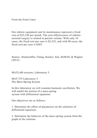
The motion of a mass suspended to a vertical spring can be described as follows. When the spring is
not loaded it has length ℓ0 (situation (a)). When a mass m is attached to its lower end it has length ℓ
(situation (b)). From the first principle of mechanics we then obtain
mg︸︷︷︸
downward weight force
+ −k(ℓ − ℓ0)︸ ︷︷ ︸
upward tension force
= 0. (L5.1)
The term g measures the gravitational acceleration (g ≃ 9.8m/s2 ≃ 32ft/s2). The quantity k is a spring
constant measuring its stiffness. We now pull downwards on the mass by an amount y and let the mass
go (situation (c)). We expect the mass to oscillate around the position y = 0. The second principle of
mechanics yields
mg︸︷︷︸
weight
+ −k(ℓ + y − ℓ0)︸ ︷︷ ︸
upward tension force
= m
d2(ℓ + y)
dt2︸ ︷︷ ︸
acceleration of mass
, i.e., m
d2y
dt2
+ ky = 0 (L5.2)
using (L5.1). This ODE is second-order.
(a) (b) (c) (d)
y
ℓ
ℓ0
m
k
γ
Equation (L5.2) is rewritten
d2y
dt2
+ ω20y = 0 (L5.3)
c⃝2011 Stefania Tracogna, SoMSS, ASU
MATLAB sessions: Laboratory 5
where ω20 = k/m. Equation (L5.3) models simple harmonic motion. A numerical solution with ini-
tial conditions y(0) = 0.1 meter and y′(0) = 0 (i.e., the mass is initially stretched downward 10cms
and released, see setting (c) in figure) is obtained by first reducing the ODE to first-order ODEs (see
Laboratory 4).
Let v = y′. Then v′ = y′′ = −ω20y = −4y. Also v(0) = y′(0) = 0. The following MATLAB program
implements the problem (with ω0 = 2).
function LAB05ex1
m = 1; % mass [kg]
k = 4; % spring constant [N/m]
omega0 = sqrt(k/m);
y0 = 0.1; v0 = 0; % initial conditions
[t,Y] = ode45(@f,[0,10],[y0,v0],[],omega0); % solve for 0<t<10
y = Y(:,1); v = Y(:,2); % retrieve y, v from Y
figure(1); plot(t,y,’b+-’,t,v,’ro-’); % time series for y and v
grid on;
%-----------------------------------------
function dYdt = f(t,Y,omega0)
y = Y(1); v = Y(2);
dYdt = [ v ; -omega0^2*y ];
Note that the parameter ω0 was passed as an argument to ode45 rather than set to its value ω0 = 2
directly in the funct ...
Measures of Dispersion and Variability: Range, QD, AD and SD
From the Front LinesOur robotic equipment and its maintenanc.docx
1. From the Front Lines
Our robotic equipment and its maintenance represent a fixed
cost of $23,320 per month. The cost-effectiveness of robotic-
assisted surgery is related to patient volume: With only 10
cases, the fixed cost per case is $2,332, and with 40 cases, the
fixed cost per case is $583.
Source: Alemozaffar, Chang, Kacker, Sun, DeWolf, & Wagner
(2013).
MATLAB sessions: Laboratory 5
MAT 275 Laboratory 5
The Mass-Spring System
In this laboratory we will examine harmonic oscillation. We
will model the motion of a mass-spring
system with differential equations.
Our objectives are as follows:
1. Determine the effect of parameters on the solutions of
differential equations.
2. Determine the behavior of the mass-spring system from the
graph of the solution.
2. 3. Determine the effect of the parameters on the behavior of the
mass-spring.
The primary MATLAB command used is the ode45 function.
Mass-Spring System without Damping
The motion of a mass suspended to a vertical spring can be
described as follows. When the spring is
not loaded it has length ℓ0 (situation (a)). When a mass m is
attached to its lower end it has length ℓ
(situation (b)). From the first principle of mechanics we then
obtain
mg︸︷︷︸
downward weight force
+ −k(ℓ − ℓ0)︸ ︷︷ ︸
upward tension force
= 0. (L5.1)
The term g measures the gravitational acceleration (g ≃ 9.8m/s2
≃ 32ft/s2). The quantity k is a spring
constant measuring its stiffness. We now pull downwards on the
mass by an amount y and let the mass
go (situation (c)). We expect the mass to oscillate around the
position y = 0. The second principle of
mechanics yields
mg︸︷︷︸
weight
+ −k(ℓ + y − ℓ0)︸ ︷︷ ︸
upward tension force
3. = m
d2(ℓ + y)
dt2︸ ︷︷ ︸
acceleration of mass
, i.e., m
d2y
dt2
+ ky = 0 (L5.2)
using (L5.1). This ODE is second-order.
(a) (b) (c) (d)
y
ℓ
ℓ0
m
k
γ
Equation (L5.2) is rewritten
d2y
dt2
+ ω20y = 0 (L5.3)
c⃝2011 Stefania Tracogna, SoMSS, ASU
4. MATLAB sessions: Laboratory 5
where ω20 = k/m. Equation (L5.3) models simple harmonic
motion. A numerical solution with ini-
tial conditions y(0) = 0.1 meter and y′(0) = 0 (i.e., the mass is
initially stretched downward 10cms
and released, see setting (c) in figure) is obtained by first
reducing the ODE to first-order ODEs (see
Laboratory 4).
Let v = y′. Then v′ = y′′ = −ω20y = −4y. Also v(0) = y′(0) = 0.
The following MATLAB program
implements the problem (with ω0 = 2).
function LAB05ex1
m = 1; % mass [kg]
k = 4; % spring constant [N/m]
omega0 = sqrt(k/m);
y0 = 0.1; v0 = 0; % initial conditions
[t,Y] = ode45(@f,[0,10],[y0,v0],[],omega0); % solve for 0<t<10
y = Y(:,1); v = Y(:,2); % retrieve y, v from Y
figure(1); plot(t,y,’b+-’,t,v,’ro-’); % time series for y and v
grid on;
%-----------------------------------------
5. function dYdt = f(t,Y,omega0)
y = Y(1); v = Y(2);
dYdt = [ v ; -omega0^2*y ];
Note that the parameter ω0 was passed as an argument to ode45
rather than set to its value ω0 = 2
directly in the function f. The advantage is that its value can
easily be changed in the driver part of the
program rather than in the function, for example when multiple
plots with different values of ω0 need
to be compared in a single MATLAB figure window.
0 1 2 3 4 5 6 7 8 9 10
−0.2
−0.15
−0.1
−0.05
0
0.05
0.1
0.15
0.2
Figure L5a: Harmonic motion
1. From the graph in Fig. L5a answer the following questions.
6. (a) Which curve represents y = y(t)? How do you know?
(b) What is the period of the motion? Answer this question first
graphically (by reading the
period from the graph) and then analytically (by finding the
period using ω0).
(c) We say that the mass comes to rest if, after a certain time,
the position of the mass remains
within an arbitrary small distance from the equilibrium position.
Will the mass ever come to
rest? Why?
c⃝2011 Stefania Tracogna, SoMSS, ASU
MATLAB sessions: Laboratory 5
(d) What is the amplitude of the oscillations for y?
(e) What is the maximum velocity (in magnitude) attained by
the mass, and when is it attained?
Make sure you give all the t-values at which the velocity is
maximum and the corresponding
maximum value. The t-values can be determined by magnifying
the MATLAB figure using
the magnify button , and by using the periodicity of the velocity
function.
(f) How does the size of the mass m and the stiffness k of the
spring affect the motion?
Support your answer first with a theoretical analysis on how ω0
– and therefore the period
7. of the oscillation – is related to m and k, and then graphically
by running LAB05ex1.m first
with m = 5 and k = 4 and then with m = 1 and k = 16. Include
the corresponding graphs.
2. The energy of the mass-spring system is given by the sum of
the potential energy and kinetic
energy. In absence of damping, the energy is conserved.
(a) Plot the quantity E = 1
2
mv2 + 1
2
ky2 as a function of time. What do you observe? (pay close
attention to the y-axis scale and, if necessary, use ylim to get a
better graph). Does the graph
confirm the fact that the energy is conserved?
(b) Show analytically that dE
dt
= 0.(Note that this proves that the energy is constant).
(c) Plot v vs y (phase plot). Does the curve ever get close to the
origin? Why or why not? What
does that mean for the mass-spring system?
Mass-Spring System with Damping
When the movement of the mass is damped due to viscous
effects (e.g., the mass moves in a cylinder
containing oil, situation (d)), an additional term proportional to
the velocity must be added. The
resulting equation becomes
8. m
d2y
dt2
+ c
dy
dt
+ ky = 0 or
d2y
dt2
+ 2p
dy
dt
+ ω20y = 0 (L5.4)
by setting p = c
2m
. The program LAB05ex1 is updated by modifying the function
f:
function LAB05ex1a
m = 1; % mass [kg]
k = 4; % spring constant [N/m]
c = 1; % friction coefficient [Ns/m]
9. omega0 = sqrt(k/m); p = c/(2*m);
y0 = 0.1; v0 = 0; % initial conditions
[t,Y] = ode45(@f,[0,10],[y0,v0],[],omega0,p); % solve for
0<t<10
y = Y(:,1); v = Y(:,2); % retrieve y, v from Y
figure(1); plot(t,y,’b+-’,t,v,’ro-’); % time series for y and v
grid on;
%-------------------------------------------
function dYdt = f(t,Y,omega0,p)
y = Y(1); v = Y(2);
dYdt = [ v ; ?? ]; % fill-in dv/dt
3. Fill in LAB05ex1a.m to reproduce Fig. L5b and then answer
the following questions.
(a) For what minimal time t1 will the mass-spring system
satisfy |y(t)| < 0.01 for all t > t1? You
can answer the question either by magnifying the MATLAB
figure using the magnify button
(include a graph that confirms your answer), or use the
following MATLAB commands
(explain):
c⃝2011 Stefania Tracogna, SoMSS, ASU
10. MATLAB sessions: Laboratory 5
0 1 2 3 4 5 6 7 8 9 10
−0.2
−0.15
−0.1
−0.05
0
0.05
0.1
0.15
0.2
y(t)
v(t)=y’(t)
Figure L5b: Damped harmonic motion
for i=1:length(y)
m(i)=max(abs(y(i:end)));
end
i = find(m<0.01); i = i(1);
disp([’|y|<0.01 for t>t1 with ’ num2str(t(i-1)) ’<t1<’
num2str(t(i))])
11. (b) What is the maximum (in magnitude) velocity attained by
the mass, and when is it attained?
Answer by using the magnify button and include the
corresponding picture.
(c) How does the size of c affect the motion? To support your
answer, run the file LAB05ex1.m
for c = 2, c = 4, c = 6 and c = 8. Include the corresponding
graphs with a title indicating
the value of c used.
(d) Determine analytically the smallest (critical) value of c such
that no oscillation appears in
the solution.
4. (a) Plot the quantity E = 1
2
mv2 + 1
2
ky2 as a function of time. What do you observe? Is the
energy conserved in this case?
(b) Show analytically that dE
dt
< 0 for c > 0 while dE
dt
> 0 for c < 0.
(c) Plot v vs y (phase plot). Comment on the behavior of the
curve in the context of the motion
of the spring. Does the graph ever get close to the origin? Why
12. or why not?
c⃝2011 Stefania Tracogna, SoMSS, ASU
function LAB05ex1a
m = 1; % mass [kg]
k = 4; % spring constant [N/m]
c = 1; % friction coefficient [Ns/m]
omega0 = sqrt(k/m); p = c/(2*m);
y0 = 0.1; v0 = 0; % initial conditions
[t,Y]=ode45(@f,[0,10],[y0,v0],[],omega0,p); % solve for
0<t<10
y=Y(:,1); v=Y(:,2); % retrieve y, v from Y
figure(1); plot(t,y,'b+-',t,v,'ro-'); % time series for y and v
grid on
%------------------------------------------------------
function dYdt= f(t,Y,omega0,p)
y = Y(1); v= Y(2);
dYdt = [v; ?? ]; % fill-in dv/dt
13. function LAB05ex1
m = 1; % mass [kg]
k = 4; % spring constant [N/m]
omega0=sqrt(k/m);
y0=0.1; v0=0; % initial conditions
[t,Y]=ode45(@f,[0,10],[y0,v0],[],omega0); % solve for 0<t<10
y=Y(:,1); v=Y(:,2); % retrieve y, v from Y
figure(1); plot(t,y,'b+-',t,v,'ro-'); % time series for y and v
grid on;
%------------------------------------------------------
function dYdt= f(t,Y,omega0)
y = Y(1); v= Y(2);
dYdt = [v; -omega0^2*y];
14. MATLAB sessions: Laboratory 5
MAT 275 Laboratory 5
The Mass-Spring System
In this laboratory we will examine harmonic oscillation. We
will model the motion of a mass-spring
system with differential equations.
Our objectives are as follows:
1. Determine the effect of parameters on the solutions of
differential equations.
2. Determine the behavior of the mass-spring system from the
graph of the solution.
3. Determine the effect of the parameters on the behavior of the
mass-spring.
The primary MATLAB command used is the ode45 function.
Mass-Spring System without Damping
The motion of a mass suspended to a vertical spring can be
described as follows. When the spring is
not loaded it has length ℓ0 (situation (a)). When a mass m is
attached to its lower end it has length ℓ
(situation (b)). From the first principle of mechanics we then
obtain
mg︸︷︷︸
downward weight force
15. + −k(ℓ − ℓ0)︸ ︷︷ ︸
upward tension force
= 0. (L5.1)
The term g measures the gravitational acceleration (g ≃ 9.8m/s2
≃ 32ft/s2). The quantity k is a spring
constant measuring its stiffness. We now pull downwards on the
mass by an amount y and let the mass
go (situation (c)). We expect the mass to oscillate around the
position y = 0. The second principle of
mechanics yields
mg︸︷︷︸
weight
+ −k(ℓ + y − ℓ0)︸ ︷︷ ︸
upward tension force
= m
d2(ℓ + y)
dt2︸ ︷︷ ︸
acceleration of mass
, i.e., m
d2y
dt2
+ ky = 0 (L5.2)
using (L5.1). This ODE is second-order.
(a) (b) (c) (d)
y
16. ℓ
ℓ0
m
k
γ
Equation (L5.2) is rewritten
d2y
dt2
+ ω20y = 0 (L5.3)
c⃝2011 Stefania Tracogna, SoMSS, ASU
MATLAB sessions: Laboratory 5
where ω20 = k/m. Equation (L5.3) models simple harmonic
motion. A numerical solution with ini-
tial conditions y(0) = 0.1 meter and y′(0) = 0 (i.e., the mass is
initially stretched downward 10cms
and released, see setting (c) in figure) is obtained by first
reducing the ODE to first-order ODEs (see
Laboratory 4).
Let v = y′. Then v′ = y′′ = −ω20y = −4y. Also v(0) = y′(0) = 0.
The following MATLAB program
implements the problem (with ω0 = 2).
function LAB05ex1
17. m = 1; % mass [kg]
k = 4; % spring constant [N/m]
omega0 = sqrt(k/m);
y0 = 0.1; v0 = 0; % initial conditions
[t,Y] = ode45(@f,[0,10],[y0,v0],[],omega0); % solve for 0<t<10
y = Y(:,1); v = Y(:,2); % retrieve y, v from Y
figure(1); plot(t,y,’b+-’,t,v,’ro-’); % time series for y and v
grid on;
%-----------------------------------------
function dYdt = f(t,Y,omega0)
y = Y(1); v = Y(2);
dYdt = [ v ; -omega0^2*y ];
Note that the parameter ω0 was passed as an argument to ode45
rather than set to its value ω0 = 2
directly in the function f. The advantage is that its value can
easily be changed in the driver part of the
program rather than in the function, for example when multiple
plots with different values of ω0 need
to be compared in a single MATLAB figure window.
0 1 2 3 4 5 6 7 8 9 10
−0.2
18. −0.15
−0.1
−0.05
0
0.05
0.1
0.15
0.2
Figure L5a: Harmonic motion
1. From the graph in Fig. L5a answer the following questions.
(a) Which curve represents y = y(t)? How do you know?
(b) What is the period of the motion? Answer this question first
graphically (by reading the
period from the graph) and then analytically (by finding the
period using ω0).
(c) We say that the mass comes to rest if, after a certain time,
the position of the mass remains
within an arbitrary small distance from the equilibrium position.
Will the mass ever come to
rest? Why?
c⃝2011 Stefania Tracogna, SoMSS, ASU
19. MATLAB sessions: Laboratory 5
(d) What is the amplitude of the oscillations for y?
(e) What is the maximum velocity (in magnitude) attained by
the mass, and when is it attained?
Make sure you give all the t-values at which the velocity is
maximum and the corresponding
maximum value. The t-values can be determined by magnifying
the MATLAB figure using
the magnify button , and by using the periodicity of the velocity
function.
(f) How does the size of the mass m and the stiffness k of the
spring affect the motion?
Support your answer first with a theoretical analysis on how ω0
– and therefore the period
of the oscillation – is related to m and k, and then graphically
by running LAB05ex1.m first
with m = 5 and k = 4 and then with m = 1 and k = 16. Include
the corresponding graphs.
2. The energy of the mass-spring system is given by the sum of
the potential energy and kinetic
energy. In absence of damping, the energy is conserved.
(a) Plot the quantity E = 1
2
mv2 + 1
2
ky2 as a function of time. What do you observe? (pay close
attention to the y-axis scale and, if necessary, use ylim to get a
20. better graph). Does the graph
confirm the fact that the energy is conserved?
(b) Show analytically that dE
dt
= 0.(Note that this proves that the energy is constant).
(c) Plot v vs y (phase plot). Does the curve ever get close to the
origin? Why or why not? What
does that mean for the mass-spring system?
Mass-Spring System with Damping
When the movement of the mass is damped due to viscous
effects (e.g., the mass moves in a cylinder
containing oil, situation (d)), an additional term proportional to
the velocity must be added. The
resulting equation becomes
m
d2y
dt2
+ c
dy
dt
+ ky = 0 or
d2y
dt2
+ 2p
21. dy
dt
+ ω20y = 0 (L5.4)
by setting p = c
2m
. The program LAB05ex1 is updated by modifying the function
f:
function LAB05ex1a
m = 1; % mass [kg]
k = 4; % spring constant [N/m]
c = 1; % friction coefficient [Ns/m]
omega0 = sqrt(k/m); p = c/(2*m);
y0 = 0.1; v0 = 0; % initial conditions
[t,Y] = ode45(@f,[0,10],[y0,v0],[],omega0,p); % solve for
0<t<10
y = Y(:,1); v = Y(:,2); % retrieve y, v from Y
figure(1); plot(t,y,’b+-’,t,v,’ro-’); % time series for y and v
grid on;
%-------------------------------------------
function dYdt = f(t,Y,omega0,p)
22. y = Y(1); v = Y(2);
dYdt = [ v ; ?? ]; % fill-in dv/dt
3. Fill in LAB05ex1a.m to reproduce Fig. L5b and then answer
the following questions.
(a) For what minimal time t1 will the mass-spring system
satisfy |y(t)| < 0.01 for all t > t1? You
can answer the question either by magnifying the MATLAB
figure using the magnify button
(include a graph that confirms your answer), or use the
following MATLAB commands
(explain):
c⃝2011 Stefania Tracogna, SoMSS, ASU
MATLAB sessions: Laboratory 5
0 1 2 3 4 5 6 7 8 9 10
−0.2
−0.15
−0.1
−0.05
0
0.05
0.1
23. 0.15
0.2
y(t)
v(t)=y’(t)
Figure L5b: Damped harmonic motion
for i=1:length(y)
m(i)=max(abs(y(i:end)));
end
i = find(m<0.01); i = i(1);
disp([’|y|<0.01 for t>t1 with ’ num2str(t(i-1)) ’<t1<’
num2str(t(i))])
(b) What is the maximum (in magnitude) velocity attained by
the mass, and when is it attained?
Answer by using the magnify button and include the
corresponding picture.
(c) How does the size of c affect the motion? To support your
answer, run the file LAB05ex1.m
for c = 2, c = 4, c = 6 and c = 8. Include the corresponding
graphs with a title indicating
the value of c used.
(d) Determine analytically the smallest (critical) value of c such
that no oscillation appears in
the solution.
4. (a) Plot the quantity E = 1
24. 2
mv2 + 1
2
ky2 as a function of time. What do you observe? Is the
energy conserved in this case?
(b) Show analytically that dE
dt
< 0 for c > 0 while dE
dt
> 0 for c < 0.
(c) Plot v vs y (phase plot). Comment on the behavior of the
curve in the context of the motion
of the spring. Does the graph ever get close to the origin? Why
or why not?
c⃝2011 Stefania Tracogna, SoMSS, ASU