1. 4-10
4.2.5 Infeasible solution
In case of c 'T ≥ 0, but at least one element of b 'i is negative. The algorithm will
N
be terminated (step 1). But all basic variables can not be negative.
4.3 The Simplex Method in Tabular Form
The tabular form of the simplex method is mathematically equivalent to the
algebraic form. Instead of writing down each set of equations in full detail, we use a
simplex tableau to record only the essential information, namely, (1) the coefficients of
the basic variables, (2) the constants on the right-hand side of equations, and (3) the basic
variables appearing in each equation.
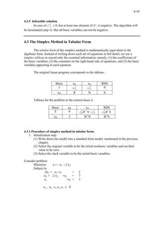
The original linear program corresponds to the tableau :
Basic xB xN RHS
z T
- cB - cT
N
0
xB B N b
Tableau for the problem in the current basis is
Basic xB xN RHS
Z 0 −1
c B N − cT
T
B N cB B −1b
T
-1
xB I B N B-1b
4.3.1 Procedure of simplex method in tabular form:
1. Initialization step:
(1) Write down the model into a standard form model, mentioned in the previous
chapter.
(2) Select the original variable to be the initial nonbasic variables and set their
value to be zero.
(3) Select the slack variable to be the initial basic variables.
Consider problem
Minimize z = - x1 - 2 x2
Subject to
-2x1 + x2 +s1 = 2
-x1 + 2 x2 +s2 = 7
x1 +s3 = 3
x1 , x2, s1, s2, s3 ≥ 0

2. 4-11
The initial tabular is
Basic x1 x2 s1 s2 s3 RHS
z 1 2 0 0 0 0
s1 -2 1 1 0 0 2
s2 -1 2 0 1 0 7
s3 1 0 0 0 1 3
2. Optimality Test:
The current basic solution is optimal if and only if every coefficient in the first
row of table (Z’s row) is ≤ 0. If it is, then stop; otherwise, go to the iterative step
to obtain the next basic feasible solution. In this example the initial tabular above,
coefficients of x1 and x2 are positive. Thus go to the iterative step.
3. Iterative Step:
(1) Determine the entering basic variable by selecting the variable with the
positive coefficient having the largest value in the first row (Z’s row). The
column below this coefficient is called the pivot column. In this example the
column of x2 is the pivot.
Basic x1 x2 s1 s2 s3 RHS
Z 1 2 0 0 0 0
s1 -2 1 1 0 0 2
s2 -1 2 0 1 0 7
s3 1 0 0 0 1 3
(2) Determine the leaving basic variable by (1) picking out each coefficient in the
pivot column that is positive (>0), (2) dividing each of these coefficients into
“right hand side” for the same row, (3) identifying the equation that has
smallest of this ratios, and (4) selecting the basic variable for this equation.
For this example, the ratios for row 1 to row 3 are :
Row 1 : 2/1 = 2
Row 2: 7/2 = 3.5
Row 3: -
Row 1 has the smallest ratio. Thus, choose the s1 to leave the basis.
(3) Put a box around this equation’s row in the tabular to the right of z column.
This row is called pivot row and one number in these boxes is also called the
pivot number.
For example the first row (the row of s1 ) is pivot row and “1” is the pivot
number.
Basic x1 x2 s1 s2 s3 RHS
z 1 2 0 0 0 0
s1 -2 1 1 0 0 2
s2 -1 2 0 1 0 7
s3 1 0 0 0 1 3

3. 4-12
(4) Determine the new feasible solution by constructing a new simplex tabular in
proper from Gaussian elimination below the current one.
Basic x1 x2 s1 s2 s3 RHS
z -5 0 2 0 0 4
s1 -2 1 1 0 0 2
s2 3 0 -2 1 0 3
s3 1 0 0 0 1 3
Then perform return to step 2.
4.3.2 Tie Breaking in the simplex method
(1) Tie for the entering basic variable
In step of determining the entering variable, it the objective function is
z = - 4x1 - 4 x2. The coefficients of x1 and x2 are equal. The selection between
these two variables can be made arbitrarily. The optimal solution will be
reached eventually.
(2) Tie for the leaving basic variable (degeneracy)
In step of determining the leaving variable, the minimum ratio of right side
and the coefficient in pivot column for the two variables are equal. Choosing
one variable to be the leaving basis variable would lead the other one being
zero in the new basis solution.
(3) No leaving basic variable (unbounded z)
In step of determining the leaving variable, no variable qualifies to be the
leaving basis variable. This means that every coefficient in the pivot column
(excluding z’row) is either zero or negative. This result would occur if the
entering basic variable could be increased indefinitely without giving negative
values to any of the current basis.
(4) Multiple optimal solution
Since the tabular simplex method will be stop after reaching one optimal
solution. In order to test whether the multiple optimal solutions exist. After
getting the optimal solution, perform the extra iteration by force one nonbasic
variable into the basis. If the solution is still feasible, there are multiple
solutions (since there are no changes in the coefficients of variables in the z’s
row and objective value).

4. 4-13
Example 4.5 : Consider the Table below
Iteration Basic Coefficients of RHS
Vars. x1 x2 s1 s2 s3
2 z 0 0 0 0 -1 18
x1 1 0 1 0 0 4
s2 0 0 3 1 -1 6
x2 0 1 -3/2 0 1/2 3
extra z 0 0 0 0 -1 18
x1 1 0 0 -1/3 1/3 2
s1 0 0 1 1/3 -1/3 2
x2 0 1 0 1/2 0 6
4.4 Revised the Simplex Method
The revised simplex method is a systematic procedure for implementing the step
for the simplex method in a smaller array. Therefore it is saving the storage space.
Form of the simplex method creates at each iteration only the information that is
specifically required for that iteration. The result is a version of the method, which
requires less storage and less computation.
Consider the final tabular:
Basic xB xN rhs
z 0 T
B
−1
c B N − cT
N c B −1b
T
B
-1
xB I B N B-1b
To generate the revised simplex version, both of the matrix B-1and original
information are required.
If the basis matrix inverse B-1 is available, then
xB = b’ = B-1 b
and the associated objective value is
z ' = cB B −1b = cB xB
T T
The columns of the current tabular, A’j are obtained from
A’j = B-1 Aj Where Aj is the jth column of A
Let yT = cB B −1 , the reduced cost will be c’j = c’j - yT Aj
T
The revised simplex tableau is a tool for updating the inverse of the basis matrix.
At each iteration, the m×m matrix B-1 and three vectors: right-hand-side, y and the
entering column are needed. Thus, we will focus on only these components from
the simplex tableau. The reduced tableau is called revised simplex or inverse
tableau.

5. 4-14
basic inverse RHS
z yT T
cB b '
xB1 b’1
… …
xBs B-1 b’s
… …
xBm b’m