2. 208 Leonardo L. Giovanini / ISA Transactions 42 (2003) 207–226
predict the system output at its steady-state value 2. Single-step output predictor
͑prediction time is set equal to the convolution
length͒ and then develop the controller structure. In many predictive control techniques, the
On the other hand, APA predicts the controlled model more frequently used to develop the predic-
variable on dead time plus one sample and then tor is the discrete convolution truncated to N terms
uses the predicted error as input into the controller. ͓4,9͔. The reason is twofold: ͑a͒ the convolution
Finally, VHP uses the predicted error as the input summation gives the model output explicitly and
into the controller, like APA, but the prediction ͑b͒ the main impulse response coefficients are
can be freely chosen from the hole prediction ho- relatively easy to obtain. In particular, for single-
rizon and it does not impose any constraint on the input/single-output ͑SISO͒ systems
controller that can be used. N
In this work a new method for designing a y ͑ J,k ͒ ϭ ͚ ˜ i u ͑ kϩJϪi ͒ ,
ˆ h JϽN, ͑1͒
predictive is presented. The approach is based on iϭ1
the use of only one prediction of the system out-
put, instead of the complete trajectory: it uses a predicts the output value J sampling intervals
ahead, k represents the current time instant t
prediction of the process output J time inter-
vals ahead to compute the correspondent future ϭkt S ( t S is the sampling interval͒, ˜ i , i h
error. The proposed controller, called predictive ϭ1,2, . . . ,N are the impulse response coefficients,
feedback controller, uses the last w predicted and u ( kϩJϪi ) , iϭ1,2,...,N is the sequence of
errors instead of using plain feedback errors, as inputs to be considered. However, most frequently
in classical feedback controllers. Hence the re- y ( J,k ) is not calculated directly from Eq. ͑1͒ but
ˆ
from a modified expression that includes the pre-
sulting control action is computed by observ-
diction for the current time y ( 0,k ) . For this, notice
ˆ
ing the system future behavior and also by
that Eq. ͑1͒ can also be written as a function of the
weighting present and past errors. So, this control
predicted value for the previous sampling time J
strategy combines the predictive capacity, which
Ϫ1,
results in good performance for set-point
changes and time delay systems, with the classical N
use of the feedback information which imp- y ͑ J,k ͒ ϭy ͑ JϪ1,k ͒ ϩ ͚ ˜ i ⌬u ͑ kϩJϪi ͒ ,
ˆ ˆ h
iϭ1
roves the system performance for disturbance
͑2͒
rejection.
The organization of the paper is as follow: in where ⌬u ( kϩJϪi ) ϭu ( kϩJϪi ) Ϫu ( kϩJϪi
Section 2 the expressions for a general J -step Ϫ1 ) . Then, successive substitutions of y ( J
ˆ
ahead output prediction are presented. In Section 3 Ϫ1,k ) by previous predictions gives
the basic formulation for the single-prediction
J N
controller design is derived. Furthermore, a rela-
tionship between the controller parameter and the y ͑ J,k ͒ ϭy ͑ 0,k ͒ ϩ ͚
ˆ ˆ ͚ ˜ i ⌬u ͑ kϩlϪi ͒ .
h
lϭ1 iϭ1
settling time of closed-loop response is estab- ͑3͒
lished. In Section 4 the closed-loop stability and
performance of the single-prediction controller are This equation defines a J -step ahead predictor,
analyzed. In Section 5 a direct feedback mode is which includes future control actions. Since future
introduced in order to improve the overall system control actions are unknown, the predictor ͑3͒ is
performance. Besides, the relationship between not realizable. To turn it realizable a statement
the proposed controller and other predictive con- must be made about how the control variable is
trol algorithms is established. The closed-loop sta- going to move in the future. For example, the sim-
bility and performance of the resulting controller plest rule is to set all of them equal to zero,
are analyzed in Section 6. In Section 7 we show ⌬u ͑ kϩ j ͒ ϭ0, ᭙ jϭ0,1,...,J, ͑4͒
the results obtained from the application of the
proposed algorithm to a nonlinear continuous which implies that the control variable will not
stirred tank reactor. Finally, the conclusions are move in future sampling instants. Then, Eq. ͑3͒
presented in Section 8. becomes
3. Leonardo L. Giovanini / ISA Transactions 42 (2003) 207–226 209
J N 3. Single-prediction control
y ͑ J,k ͒ ϭy ͑ 0,k ͒ ϩ ͚
ˆ 0
ˆ ͚ ˜ i ⌬u ͑ kϩlϪi ͒ ,
h
lϭ1 iϭlϩ1
Although the idea of using only one prediction
͑5͒ of the system output for controlling the system is
not new ͓5– 8͔, all the authors did not use the pre-
where the superscript 0 recalls that condition ͑4͒ is
diction time J as a tuning parameter. This is the
included. The new expression ͑5͒ defines a realiz-
case of single-prediction controller, whose deriva-
able open-loop J -step ahead predictor whose Z
tion procedure is quite straightforward from the
transform is given by ͑see Appendix A͒
open-loop predictor. Revising the assumption used
to go from Eq. ͑3͒ to Eq. ͑5͒ observe that if just
y 0 ͑ J,z ͒ ϭ P ͑ J,z ͒ u ͑ z ͒ ,
ˆ ͑6͒
the control movement ⌬u ( k ) 0, then
where P ( J,z ) is the transfer function of the open- y ͑ J,k ͒ ϭy 0 ͑ J,k ͒ ϩa J ⌬u ͑ k ͒ .
ˆ ˆ ˜ ͑9͒
loop predictor given by
This prediction can be substracted from a refer-
N ence variable r ( kϩJ ) to obtain the predicted error
P ͑ J,z ͒ ϭa J z Ϫ1 ϩ
˜ ͚ ˜ i z JϪi ,
h
iϭJϩ1 e ͑ J,k ͒ ϭe 0 ͑ J,k ͒ Ϫa J ⌬u ͑ k ͒ .
ˆ ˆ ˜ ͑10͒
and ˜ J is the Jth coefficient of step response.
a The control action can be computed in the similar
The prediction y 0 ( J,k ) is updated by adding
ˆ way as standard predictive controllers, minimizing
the following performance measure,
˜ ͑ J,z ͒ ϭy ͑ J,z ͒ Ϫy ͑ J,z ͒ .
d ˆ ͑7͒
f ͑ k ͒ ϭe 2 ͑ J,k ͒ ϩ ⌬u 2 ͑ k ͒ ,
ˆ у0. ͑11͒
This term lumps together possible unmeasured Then, the control action that minimizes this per-
disturbance and inaccuracies due to plant-model formance index is given by
mismatch. Since the future value of ˜ ( J,z ) is not
d
available, an estimate is used. In the absence of 1 0
⌬u ͑ k ͒ ϭ ˆ ͑ J,k ͒ ,
e ͑12͒
any additional knowledge of ˜ ( J,z ) , the predicted
d KJ
disturbance is assumed to be equal to that esti-
where e 0 ( J,k ) ϭr ( kϩJ ) Ϫy 0 ( J,k ) and K J ϭa J
ˆ ˆ ˜
mated at the current time ˜ ( z ) . A more accurate
d
ϩ /a J , and the cost of controlling the system is
˜
estimate of ˜ ( J,z ) is possible if the disturbance
d
output model and a measure of load disturbance 2
are available. So, we use a similar equation to Eq. f ͑ k ͒ϭ ˆ 0 ͑ J,k ͒ .
e
˜ 2ϩ
aJ
͑6͒ to predict the future disturbance. The impor-
tance of the form of Eq. ͑5͒ comes also from the At this point of the work we are interested on
fact that the prediction y 0 ( J,k ) can be updated by
ˆ understanding the meaning of prediction time J
the current output measurement y ( k ) . This is done and its relationship with the closed-loop response.
by substituting y ( 0,k ) by y ( k ) , or equivalently the
ˆ To do it, we replace ⌬u ( k ) and K J in the closed-
correction is implemented by ˜ ( z ) adding to Eq.
d loop predicted error ͓Eq. ͑10͔͒, so we can write it
͑6͒, in any case we obtain as function of e 0 ( J,k ) and ,
ˆ
y 0 ͑ J,z ͒ ϭy ͑ z ͒ ϩ ͓ P ͑ J,z ͒ ϪG p ͑ z ͔͒ u ͑ z ͒ , ͑8͒
ˆ ˜
e ͑ J,k ͒ ϭ
ˆ ˆ 0 ͑ J,k ͒ .
e
˜ 2ϩ
aJ
˜
where G p ( z ) is the plant model. This equation
Then, defining e ( J,k ) as a fraction of e 0 ( J,k ) ,
ˆ ˆ
defines a realizable corrected J -step ahead predic-
tor. Hence there are two type of predictors: one is e ͑ J,k ͒ ϭ ␣ e 0 ͑ J,k ͒ ,
ˆ ˆ ͉ ␣ ͉ Ͻ1,
the open-loop predictor that only depends on the
values of the past inputs only ͓Eq. ͑6͔͒ and the where ␣ is the remaining error after the control
other is the corrected predictor ͑8͒ which receives action ⌬u ( k ) is applied, the control cost is re-
a correction through the feedback measurement. lated with ␣ through
4. 210 Leonardo L. Giovanini / ISA Transactions 42 (2003) 207–226
then assumed constant from every sampling in-
stant k into the future. In other words, given all the
input changes accounted for until the instant k, the
single-prediction controller observes the value that
would be reached by the system output if no future
control action is taken and then u ( k ) is computed
such to the performance index ͑11͒ is minimized.
Hence if ˜ ( z ) actually remains constant after the
d
instant k and ϭ0, then the output reaches the
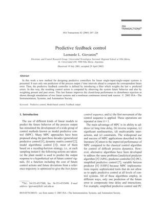
Fig. 1. Structure of the single-prediction controller. reference value J sampling intervals later.
Note that controller ͑15͒ is realizable if and only
if ˜ J 0. Then, the prediction time J should be
a
chosen such that
␣
ϭ ˜2.
a
1Ϫ ␣ J
This equation means that the closed-loop error
Jуint ͩͪtd
tS
ϩ1,
will be bounded by ͉ e ( k 0 ϩJ ) ͉ р ␣ ͉ e 0 ( J,k 0 ) ͉ , ᭙t
ˆ where t d is the process time delay. This fact means
Ͼk 0 ϩJ, where k 0 is time instant where the set- that the open-loop predictor P ( J,z ) compensates
point changes. Therefore the prediction time J the process time delay. In the following sections
could be seen as the closed-loop settling time for we assume that ϭ0 to simplify the expositions,
an error ␣ ͉ e ( k 0 ) ͉ . When the control cost is set however, the results that will be obtained are the
to 0, which is equivalent to ␣ ϭ0, the performance same whether the control weight is set to zero or
measure ͑11͒ and the predicted closed-loop error not.
e ( J,k ) becomes zero, and the control change is
ˆ
given by 4. Algorithm properties
1 0 4.1. Stability analysis
⌬u ͑ k ͒ ϭ ˆ ͑ J,k ͒ .
e ͑13͒
˜J
a
To analyze the effect of the prediction time over
On the other hand, when is set to ϱ ͑which is the closed-loop stability, we substituted the con-
equivalent to ␣ ϭ1) no control action is taken and troller ͑15͒ in the closed-loop characteristic equa-
e ( J,k ) ϭe 0 ( J,k 0 ) ϭe ( k 0 ) , ᭙kϾk 0 .
ˆ ˆ tion to obtain
Using Z transform on Eq. ͑12͒ shows that the
single predictive control algorithm is basically an ͑ 1Ϫz Ϫ1 ͒˜ J ϩ P ͑ J,z ͒ ϩ ͓ Gp ͑ z ͒ ϪG p ͑ z ͔͒ ϭ0.
a ˜
integral action applied on the predicted error
Then, combining this expression with Eqs. ͑A8͒
1 1 and ͑A2͒, and using the convolution model of the
u͑ z ͒ϭ ˆ 0 ͑ J,z ͒ .
e ͑14͒
K J 1Ϫz Ϫ1 process, this equation becomes
N N
Combining Eqs. ͑14͒ and ͑8͒ the result is the con-
troller, ˜ Jϩ
a ͚
iϭJϩ1
˜ i z JϪi ϩ ͚ ͑ h i Ϫh i ͒ z Ϫi
h
iϭ1
˜
1 ϱ
C͑ z ͒ϭ
͑ 1Ϫz Ϫ1 ͒ K J ϩ P ͑ J,z ͒ ϪG p ͑ z ͒
˜
. ϩ ͚
iϭNϩ1
h i z Ϫi ϭ0. ͑16͒
͑15͒
Using a result obtained by Desoer and Vidyasagar
Fig. 1 shows a block diagram of C ( z ) , where it is ͓10͔ for lineal discrete systems, we derive the fol-
apparent that it uses the plant model to estimate lowing stability condition ͑see Appendix B͒:
͚ͯ ͯ
the output at the present time y ( 0,k ) . This value is
ˆ N N ϱ
then compared with the actual measurement y ( k )
to detect modeling errors and external distur- ͚
iϭJϩ1
͉˜ i ͉ ϩ ͚ ͉ h i Ϫh i ͉ ϩ
h
iϭ1
˜
iϭNϩ1
h i Ͻa J .
˜
bances. The global detected disturbance ˜ ( z ) is
d ͑17͒
5. Leonardo L. Giovanini / ISA Transactions 42 (2003) 207–226 211
The left side of this equation has, ordered from left Since J stb guarantees the closed-loop stability for
to right, the following three terms: ͑a͒ the contri- all the models of W, the open-loop predictor
bution of the nominal model, ͑b͒ the additive un- P ( J,z ) can be directly built from the nonlinear
certainty, and ͑c͒ the effect of the truncation model model. This fact improves the accuracy of the
error; all of them are related with the convolution open-loop prediction and the closed-loop perfor-
length N. When there is not uncertainty in the mance. The nonlinear predictor can be built from
system and if N is large enough to neglect the the nonlinear model employing a numerical inte-
truncation error, Eq. ͑17͒ becomes gration scheme or using a local model network
N
͓11͔.
A final remark is for recalling that the stability
͚
iϭJϩ1
͉˜ i ͉ Ͻa J stb .
h ˜ ͑18͒ condition given by Desoer and Vidyasagar ͓10͔ is
a sufficient one. Consequently, stability conditions
This condition guarantees that—for any time- ͑17͒–͑19͒ become conservative and impose a too
invariant stable plant—there is always a value of J high lower bound for selecting J. So, always there
for which the closed-loop system is asymptotically are prediction times lower than J stb ; for those the
stable. We must note that if the plant has a mono- closed-loop system will be stable. The first J that
tone step response, the stability condition ͑18͒ can guarantees the closed-loop stability can be found
be written as through a direct search, because the solution space
ϱ is bounded,
1 1
˜ J stb Ͼ
a ͚ ˜ i ϭ 2 ˜ p,
2 iϭ1
h K 1рJрJ stb .
˜
where K p is the process gain. 4.2. Performance analysis
Generally, control engineers assume that a fam-
ily W of M linear models is capable to capture a The tuning of the single-prediction controller
moderate nonlinearity. Therefore to guarantee the implies a discrete optimization problem having a
stability of the system we must choose a J such bounded solution space
that it guarantees the stability of all the plants of
JN, 0рJрN.
W. Then, the robust stability problem becomes the
problem of finding a J such that Eq. ͑17͒ is satis- Hence, independently of the performance index
fied for each model of W. Using global additive being used, the general solution results from a di-
uncertainty and choosing N large enough to ne- rect search in the solution space. However, when
glect the truncation error, Eq. ͑17͒ becomes the ISE index is used, the optimal controller re-
N N sults from the solution of the following problem:
͚
iϭJϩ1
͉˜ i ͉ ϩ ͚ max ͉ h li Ϫh i ͉ Ͻa J stb . ͑19͒
h
iϭ1 l[1,M ]
˜ ˜ min ʈ e ͑ z ͒ ʈ 2 ϭ min ʈ ˜ ͑ z ͓͒ d ͑ z ͒ Ϫr ͑ z ͔͒ ʈ 2 ,
2
Gc(z) Gc(z)
Another way to solve the robust stability problem which is equivalent to minimize the sensitivity
is to find a J that satisfies simultaneously Eq. ͑18͒
function ˜ ( z ) over the whole system bandwidth,
for all the models of W. In the case of a system
with monotone response, the stability condition min ʈ ˜ ͑ z ͒ ʈ 2 ϭ min ʈ 1ϪG p ͑ z ͒ Gc ͑ z ͒ ʈ 2 ,
˜
͑19͒ can be written as Gc(z) Gc(z)
J stb ϭmax͑ J 1 ;J 2 ;...;J M ͒ , and to guarantee the internal stability of the
closed-loop system ͓12͔. Under these design con-
where J l , lϭ1,2,...,M is the prediction time for ditions the sensitivity function will be minimum
the lth model of the family W. This expression when the open-loop controller Gc ( z ) is given by
means that we can choose a different prediction
time for each model of W, then we selected the GcϭG p Ϫ1 ,
˜ ϩ
bigger prediction time.
At this point, a remark about how to build a ˜
where G p ϩ is the nonminimum phase portion of
predictor for nonlinear system must be made. the plant ͑right-half plane zeros and time delay͒.
6. 212 Leonardo L. Giovanini / ISA Transactions 42 (2003) 207–226
For the single-prediction controller, this condition
is equivalent to choose a prediction such that the
Jth coefficient of the step response ˜ J has the
a
u ͑ k ͒ ϭu ͑ kϪ1 ͒ ϩ ͚ͭ ͮ
V
jϭ1
k j e͑ k ͒
same sign as the stationary process gain, i.e., V
J ISE ϭk i ϩ1, ͑20͒ Ϫ ͚ k j ͓ P ͑ j,z ͒ ϪG p ͑ z ͔͒ u ͑ kϪ1 ͒ ,
˜
jϭ1
where k i is the number of samples which covers ͑24͒
the effect of the minimum phase portion of the
plant. where V is the prediction horizon and k j , j
When JϭJ ISE , the controller gain ˜ Ϫ1 is the
aJ ϭ1,2,...,V is the jth element of the gain vector. In
largest. Therefore it provides a vigorous control these equations we can see that both predictive
action and attempts to drive the system output to controllers have a similar structure: the two first
the reference in J ISE time intervals. In this case, terms, ordered from the left, are a discrete PI con-
the single-prediction controller becomes a dead- troller and the last term is a weighing contribution
beat ͑minimum-time͒ controller of the future open-loop deviations at time ( k
ϩ j)tS ,
1
C͑ z ͒ϭ . ⌬y 0 ͑ j,k ͒ ϭy 0 ͑ j,k ͒ Ϫy ͑ k ͒ ,
ˆ ˆ ˜ jϭ1,2,...,V,J.
Ϫ1
͑ 1Ϫz ͒˜ J ISE ϩ P ͑ J ISE ,z ͒ ϪG p ͑ z ͒
a ˜
͑21͒ They only differ in the number of prediction gains
employed. So, it is easy to see that we can choose
When J is increased the controller gain and the the prediction time J such that both predictive
closed-loop performance decreases. In case of J controllers, single-prediction and DMC, have
ϭN the controller gain is the inverse of process similar performances.
gain (˜ J ϭK p ) and the controller drives the sys-
a ˜ Example 4.1. To analyze the sensitivity of the pro-
tem output to the reference in N time intervals. posed controllers to the parameter J we consider
Thus only one significant control move is ob- a heat exchanger, whose hot outlet temperature is
served in absence of uncertainty ͑minimum- controlled by manipulating the cold stream flow
energy controller͒ and the single-prediction con- rate, modeled by [13]
troller becomes a predictor controller ͓6͔,
35.41
Gp ͑ s ͒ ϭϪ . ͑25͒
1 ͑ 4.5sϩ1 ͒ 5
C͑ z ͒ϭ . ͑22͒
˜ N ϪG p ͑ z ͒
a ˜ The discrete model employed to build the single-
prediction controller is obtained by assuming a
To finish this analysis, we give a heuristic com- zero-order hold at the input of continuous model
parison of the closed-loop performance achieved (25), a sampling time t S ϭ2 and the convolution
by the single-prediction controller with that of a length N was fixed in 50 terms. The prediction
MPC controller. To carry out this comparison we time is chosen using the stability condition (18), so
analyze the control actions computed by both con- J must be
trollers. They are obtained by replacing the open-
loop error by their components, assuming a step Jу12.
change in the setpoint, in the controller equations
͓4,9͔ and combining them with the predicted out- Fig. 2 shows the responses to a setpoint change
put ͑8͒. The result for the single-prediction con- for different values of J. As it was anticipated,
troller is small values of J give more rapid response and
require large initial movements in the control vari-
u ͑ k ͒ ϭu ͑ kϪ1 ͒ ϩK Ϫ1 e ͑ k ͒
J able (Fig. 3). Observe also that the closed-loop
system is stable even for values of J smaller than
ϪK Ϫ1 ͓ P ͑ J,z ͒ ϪG p ͑ z ͔͒ u ͑ kϪ1 ͒ ,
J
˜ the limit provided by Eq. (18).
Now, we compare the closed-loop responses
͑23͒
provided by single-prediction controllers with that
and the result for the MPC is provided by a DMC controller. The DMC control-
7. Leonardo L. Giovanini / ISA Transactions 42 (2003) 207–226 213
Fig. 2. Closed-loop responses of the linear system to a step change in the setpoint, showing the effect of the prediction
time J.
ler was designed following the tune procedure de- five samples, and the condition number of the con-
veloped by Rahul and Cooper [14]. The plant troller c was fixed to 500. The control weight
model (25) was approximated through a first- was computed using the following formula [14]:
order plus time delay model,
Gp ͑ s ͒ ϭϪ35.41
e Ϫ10.1s
12.04sϩ1
,
ϭ
U
c ͩ
3.5 ϩ2Ϫ
tS
UϪ1
2
K p ϭ3.73.
˜ ͪ
which was discretized assuming a zero-order hold Fig. 4 shows that the single-prediction control-
at the input and a sampling time t S ϭ2. The con- ler can provide a similar performance to that ob-
volution length is the same that we used to build tained by the DMC controller. This figure also
the single-prediction controller (Nϭ50). The pre- shows that J can be selected such that the perfor-
diction horizon V was set equal to the convolution mance or the robustness of the system be im-
length (VϭN), the control horizon U was fixed to proved, by reducing or increasing J.
Fig. 3. Control variable correspondent to the closed-loop responses shown in Fig. 2.
8. 214 Leonardo L. Giovanini / ISA Transactions 42 (2003) 207–226
Fig. 4. Closed-loop responses of the linear system to a step change in the setpoint, comparing the response of the DMC and
single-prediction controllers.
5. Predictive feedback control the prediction is calculated ͑Fig. 5͒. Hence the
control movement ⌬u ( k ) is given by
From the analysis of the closed-loop perfor-
mance in Section 4.2, it is clear that the single- w
⌬u ͑ k ͒ ϭ ͚ q * e 0 ͑ J,kϪ j ͒ ,
prediction controller provides a similar closed-
j ˆ ͑27͒
loop performance to a MPC controller. This fact jϭ0
means that a single-prediction controller shows a
poor closed-loop performance when disturbances
and uncertainties are present in the system, spe- where e 0 ( J,kϪ j ) is the J step ahead open-loop
ˆ
cially when they are assumed to be time invariant. error computed at time kϪ j. The predictive feed-
This is true even when the underlying system is back controller can be derived from Eq. ͑27͒, re-
time invariant ͓15͔. placing the open-loop error e 0 ( J,kϪ j ) by their
ˆ
A way to solve this problem is to introduce a components and following a similar procedure to
direct feedback mode in the computation of the obtain Eq. ͑15͒. The result is the controller
control action. This idea can be accomplished by
including a filter F ( z ) in the single-prediction
F͑ z ͒
control law ͑14͒. The filter not only includes a C͑ z ͒ϭ ,
feedback action in the predictive controller, but ͑ 1Ϫz Ϫ1 ͒ ϩF ͑ z ͓͒ P ͑ J,z ͒ ϪG p ͑ z ͔͒
˜
also introduces a new set of parameters to allow ͑28͒
more demanding performances. Since the control
law ͑14͒ includes an integral mode, F ( z ) can take
the following form: whose structure is shown in Fig. 6. We must note
that F ( z ) adds additional degrees of freedom to
w w
1 improve the closed-loop performance. This fact
F͑ z ͒ϭ ͚ q jz Ϫ jϭ ͚ q *z Ϫ j,
j ͑26͒ makes more difficult the controller design since
˜ J jϭ0
a jϭ0
now it is necessary to tune the filter parameters
where wZ is the filter order and q j , j ͓ 0,w ͔ ͑the coefficients q * , jϭ0,1,...,w and the order
j
are the new controller parameters. Since the con- w) . One way to solve this tuning problem is by
trol law ͑14͒ employs only one prediction of the using a method for a fixed-structure controller like
process future behavior, the delay operator z Ϫ j , j those proposed by Abbas and Sawyer ͓16͔ or Har-
ϭ0,1,...,w, is applied to the time instant at which ris and Mellichamp ͓17͔.
9. Leonardo L. Giovanini / ISA Transactions 42 (2003) 207–226 215
Fig. 5. General MPC and predictive feedback setups.
5.1. Relationship with other control algorithms w
1
C͑ z ͒ϭ ͚ q *z Ϫ j.
͑ 1Ϫz Ϫ1 ͒ jϭ0 j
͑29͒
It is easy to see that the structure of the predic-
tive feedback controller is a generalization of the
When the prediction time is set equal to the time
internal model control parametrization of the feed-
delay ( J d t S ϭt d , ) the open-loop predictor P ( J,z )
back controllers ͑Fig. 6͒. Depending on the value
becomes the system model without time delay, and
of the prediction time and the parameters of the
the predictive feedback controller ͑28͒ is the Smith
controller we have the different controllers that
predictor of the reduced order controller ͑29͒,
would be studied in the specialized literature.
When Jϭ1 the open-loop predictor P ( J,z ) be-
˜ F͑ z ͒
comes the system model G p ( z ) , and the predic- C͑ z ͒ϭ .
tive feedback controller ͑28͒ is a reduced order ͑ 1Ϫz Ϫ1 ͒ ϩF ͑ z ͓͒ 1Ϫz ϪJ d ͔ G p ͑ z ͒
˜
controller ͓6͔, ͑30͒
Fig. 6. Structure of the predictive feedback controller.
10. 216 Leonardo L. Giovanini / ISA Transactions 42 (2003) 207–226
In this case, the open-loop predictor only compen- This controller is derived from the predictive feed-
sates the time delay present in the system. In the back controller ͑28͒ by fixing its parameters to
case of JϭJ d ϩ1 and the parameters of the filter
1 
are free to be tuned, the predictive feedback con- wϭ1, q 0 ϭ a Ϫ1
˜ N , and q 1 ϭ ˜ Ϫ1 .
a
troller becomes the analytical predictor algorithm 1Ϫ  1Ϫ  N
͓5͔.
Observe that varying the parameters ␣ and  gov-
When the prediction time is greater than the
erns the character of these controllers influencing
time delay ( J d ϽJϽN ) , wϭ0, and q 0 ϭa Ϫ1 the
* ˜J
the speed of closed-loop response. When the pa-
resulting controller is the single-prediction con- rameters are in the lower limit (  ϭ0 and ␣ ϭ1) ,
troller, the controllers ͑33͒ and ͑34͒ become the predictor
controller ͑32͒, obtaining the open-loop response.
1 In the other case (  ϭ1 and ␣ ϭϱ) the controllers
C͑ z ͒ϭ , ͑31͒
˜ J ϩ P ͑ J,z ͒ ϪG p ͑ z ͒
a ˜ ͑34͒ and ͑33͒ become the inverse of the system
model, obtaining the minimum time response.
which was studied in the previous sections. The Varying the parameters between these limits we
character of this controller is governed by the pre- modify the characteristics of the closed-loop re-
diction time J, which directly influences the speed sponse, speeding up or slowing down the re-
of closed-loop response. For the particular choice sponse, in similar way as the single-prediction
of the prediction time JϭN, we can derive a fam- controller with the prediction time J.
ily of predictive controllers whose main character- Finally, we can see that predictive feedback con-
istic is to obtain a closed-loop response that is at trol has a strong connection and significant differ-
least as good as the normalized open-loop re- ence from VHP ͓8͔. The approach employed by
sponse. If no other design condition is demanded, both frameworks is similar. They employ one pre-
the controller ͑23͒ becomes the predictor control- diction of the system output, which can be freely
ler ͓6͔, chosen, and use the predicted error as inputs into
the controller. However, VHP by itself is a predic-
1 tive structure, not a controller, that can be added to
C͑ z ͒ϭ . ͑32͒ another control algorithm ͑for example PI, PID, or
˜ N ϪG p ͑ z ͒
a ˜ simplified predictive control͒. It is employed to
compensates time delay and interactions and pro-
a Ϫ1
Fixing the parameter of the controller q 0 ϭ ␣˜ N , vide a built-in feedforward scheme. In this way,
␣ у1, we obtain simplified model predictive con- VHP is similar to a single-prediction controller.
troller ͓7͔, Furthermore, VHP computes the whole trajectory,
like standard predictive control, and then selects
␣ one prediction.
C͑ z ͒ϭ . ͑33͒
˜ NϪ ␣ G p͑ z ͒
a ˜
The parameter ␣ provides a way to speed up the 6. Predictive feedback properties
closed-loop response and build a dead-time com-
pensation in the controller, but it does not give 6.1. Stability analysis
offset-free responses in the presence of modeling
errors. To solve this problem, Chawla et al. ͓18͔ Now, we study the effect of the filter and pre-
proposed the inclusion of a first-order filter into diction time on the closed-loop stability. Then, we
the control law such that the resultant controller is substitute the predictive feedback controller ͑28͒
the conservative model based controller, in the characteristic closed-loop equation, which
becomes
͑ 1Ϫ  z Ϫ1 ͒ T ͑ z Ϫ1 ͒ ϭ ͑ 1Ϫz Ϫ1 ͒ ϩF ͑ z Ϫ1 ͒ P ͑ J,z Ϫ1 ͒
C͑ z ͒ϭ ,
͑ 1Ϫ  ͒˜ N Ϫ ͑ 1Ϫ  z Ϫ1 ͒ G p ͑ z ͒
a ˜
ϩF ͑ z Ϫ1 ͓͒ Gp ͑ z Ϫ1 ͒ ϪG p ͑ z Ϫ1 ͔͒ .
˜
0р  Ͻ1. ͑34͒ ͑35͒
11. Leonardo L. Giovanini / ISA Transactions 42 (2003) 207–226 217
Combining the transfer function of the predictor ating region so that we obtain a similar closed-
͑A8͒ and using the discrete convolution, the char- loop response for each one of them. Then, during
acteristic equation T ( z Ϫ1 ) can be written as fol- the operation, we vary J according to the operat-
lows: ing region controlled at each sample.
w
͑ 1Ϫz Ϫ1
͒ ϩ ͚ q *˜ J z Ϫ jϪ1
j a
6.2. Performance analysis
jϭ0
w N
Finally, we analyze the effect of the filter over
ϩ ͚ q* ͚ ˜ i z JϪiϪ j the overall closed-loop performance and compare
j h
jϭ0 iϭJϩ1 the predictive feedback controller with a standard
MPC controller, such as the DMC. To carry out
w N
this analysis we compare the control action com-
ϩ ͚ q * ͚ ͑ h i Ϫh i ͒ z ϪiϪ j
j
˜ puted by both predictive controllers.
jϭ0 iϭ1
The control actions generated by the predictive
w ϱ feedback control law ͑27͒ are obtained by replac-
ϩ͚ q*
j ͚ h i z ϪiϪ j ϭ0. ͑36͒ ing the open-loop error e 0 ( J,kϪ j ) by their com-
ˆ
jϭ0 iϭNϩ1
ponents, assuming a step change in the setpoint,
The stability of the closed-loop system depends on and combining with the predicted output ͑8͒, the
both the prediction time J and the filter param- result is
eters. So, it may be tested by any usual stability w
u ͑ k ͒ ϭu ͑ kϪ1 ͒ ϩ ͚ q * e ͑ kϪ j ͒
criteria. Using the same procedure as in Appendix
B, we can derive the following stability condition: j
jϭ0
N
͚
iϭJϩ1
h
N
͉˜ i ͉ ϩ ͚ ͉ h i Ϫh i ͉ ϩ
iϭ1
˜ ͚ͯ ͯϱ
iϭNϩ1
h i Ͻa J .
˜
w
ϩ ͚ q * ͓ P ͑ J,z ͒ ϪG p ͑ z ͔͒ u ͑ kϪ j ͒ .
jϭ0
j
˜
Note that this condition is the same as that derived ͑37͒
for the single-prediction controller ͓Eq. ͑17͔͒.
However, we should note that the parameters of In this equation we must observe that the last term
the filter q * , jϭ0,1,...,w affect the closed-loop
j is a weighing contribution of the future open-loop
stability. These facts look contradictory, because it deviations at time ( kϪ jϩJ ) T S ,
is clear from the characteristic Eq. ͑35͒ that the
closed-loop stability depends simultaneously on ⌬y 0 ͑ J,kϪ j ͒ ϭy 0 ͑ J,kϪ j ͒ Ϫy ͑ kϪ j ͒ .
ˆ ˆ ˜
both. However, these results can be interpreted as
follows: the closed-loop stability for the predictive It only depends on the past control actions and the
feedback controller is obtained by the independent system model, so it states the effect of the past
selection of the prediction time J and the param- control actions on the future behavior of the sys-
eters of the filter, such that they independently tem. This fact implies that it has significant influ-
guarantee the closed-loop stability. These facts ence on the closed-loop performance when we
mean that the prediction time J should be selected have to track the setpoint. However, this term has
like the single-prediction controller ͓Eqs. ͑17͒ to a negligible influence when we have to reject a
͑19͔͒, and the filter must be tuned as there is no disturbance, because it has little information about
time delay in the system, because it has been com- the disturbance. The two first terms of Eq. ͑37͒,
pensated by the open-loop predictor. ordered from the left, are the time implementation
Since the prediction time J can be fixed inde- of a reduced order controller of order w ͓6͔, and
pendently of the filter’s parameters, we can vary it commands the system behavior during the distur-
such that the closed-loop performance is im- bance rejection. It is clear now that the control law
proved. Varying J we modify the closed-loop set- ͑37͒ includes a direct feedback action based on
tling time, speeding up or slowing down the sys- measured error.
tem response. So, if we have to control a nonlinear Now, we compare the performance achieved by
system we can choose a different J for each oper- the predictive feedback with that of an MPC con-
12. 218 Leonardo L. Giovanini / ISA Transactions 42 (2003) 207–226
Table 1
Predictive controller parameters and results.
Controller parameters f Set f Dist
Nϭ60, Vϭ54, Uϭ4, ϭ0.14 7.7164 3.0323
wϭ1; qϭ ͓ 0.7280 0.0987͔ 7.7061 2.5029
wϭ2; qϭ ͓ 0.7468 0.0825 0.0902͔ 7.6938 2.4595
wϭ3; qϭ ͓ 0.7614 0.0979 0.0792 0.0816͔ 7.7005 2.4229
troller. Recalling Eq. ͑24͒ we have the control ac- point tracking and disturbance rejection. To evalu-
tion generated by a standard MPC controller, ate the closed-loop responses we consider the fol-
͚ͭ ͮ
V lowing linear plant:
u ͑ k ͒ ϭu ͑ kϪ1 ͒ ϩ k j e͑ k ͒ e Ϫ50s
jϭ1
Gp ͑ s ͒ ϭ ,
͑ 150sϩ1 ͒͑ 25sϩ1 ͒
V
Ϫ ͚ k j ͓ P ͑ j,z ͒ ϪG p ͑ z ͔͒ u ͑ kϪ1 ͒ .
˜ which was used by Rahul and Cooper to evaluate
jϭ1
a tuning procedure for a DMC controller. The dis-
͑38͒ crete transfer function is obtained by assuming a
zero-order hold at the input and a sampling time
In this equation we can see that MPC controllers t S ϭ16. The tuning parameters for the DMC con-
only use the last measured error and the two first troller are same as those using by Rahul and Coo-
terms, ordered from the left, are a discrete PI con- per in his work [14] (see Table 1).
troller. Like the predictive feedback controller, the The predictive feedback controller was designed
last term is a weighing contribution of the future by solving the basic tuning problem proposed by
open-loop deviations at time ( kϩ j ) t S , j Giovanini and Marchetti [19] with the objective
ϭ1,2,...,V. function
Comparing Eqs. ͑37͒ and ͑38͒ we can see that
N
predictive feedback controller uses more feedback
information than standard predictive controllers to f ϭ ͚ e 2 ͑ k ͒ ϩ⌬u 2 ͑ k ͒ , ͑39͒
kϭ1
compute the control actions. Therefore the predic-
tive feedback controller reduces the effect of dis- for given filter orders and a prediction time (Jϭ5).
turbances more aggressively than any standard The order of the filter as chosen such that the re-
MPC controller, and has better performance than sulting controllers include the predictive version
MPC, especially for disturbance rejection problem of popular PI and PID controllers (wϭ1,2,3). The
or important uncertainties present in the system. problem described to this point has a fast solution
A final comment about the predictive feedback using an algorithm based on the descendent gra-
can be made. From Eq. ͑37͒ it is easy to see that a dient method. The filter parameters obtained for
predictive feedback controller combines the ca- each controller are shown in Table 1.
pacity of the predictive control algorithm for good The results obtained in the simulations are sum-
setpoint tracking and time delay compensation, marized in Figs. 7 and 8. They show the perfor-
with the classical use of the feedback information mance achieved by the predictive controllers nor-
to improve the disturbance rejection. Furthermore, malized to DMC performance. It has been
for controlling a nonlinear system the prediction computed as
time J can be varied to improve the closed-loop
performance by modifying the closed-loop settling f DM C x Ϫ f PF x
time. x ϭ100 , xϭSet,Dist,
f DM C x
Example 6.1. In this example we compare the
performances achieved by a predictive feedback where f DM C x , f PF,x is the performance achieved
controller and a standard MPC controller for set- by DMC and predictive feedback controllers for
13. Leonardo L. Giovanini / ISA Transactions 42 (2003) 207–226 219
Fig. 7. Performance comparison between DMC and predictive feedback, using index ͑39͒.
setpoint tracking and disturbance rejection. Fig. 7 7. Simulations and results
shows the normalized performance measured with
Eq. (39), while Fig. 8 shows the normalized per- Let us consider the problem of controlling a
formance measured with the ISE index. The pre- continuously stirred tank reactor ͑CSTR͒ in which
dictive feedback controller exhibits a similar per- an irreversible exothermic reaction is carried out
formance to the DMC controller (Fig. 7) for the at constant volume ͑Appendix C͒. This is a non-
setpoint tracking. Although a better response is linear system previously used by Morningred et
obtained by the predictive feedback controller al. ͓20͔ for testing predictive control algorithms.
(Fig. 8), it uses more control energy than DMC Fig. 9 shows the dynamic responses to the follow-
(Fig. 7). On the other hand, the predictive feed- ing sequence of changes in the manipulated vari-
back controller shows an important improvement able q c : ϩ10, Ϫ10, Ϫ10, and ϩ10 l minϪ1 ,
in the closed-loop performance for disturbance re- where the nonlinear nature of the system is appar-
jection. A better response is again obtained by
ent.
predictive feedback controller (Fig. 8) and the
Four continuous linear models are determined
controller uses a similar control energy than the
using least-squared procedures to adjust the com-
DMC (Fig. 7).
Fig. 8. Performance comparison between DMC and predictive feedback using the ISE index.
14. 220 Leonardo L. Giovanini / ISA Transactions 42 (2003) 207–226
Fig. 9. Open-loop responses of the CSTR concentration to step changes in the coolant flow rate q C (t).
position responses to the above four step changes actor using the polytope idea. These models are
in the manipulated variable. Notice that those obtained by Z transforming the continuous trans-
changes imply three different operating points cor- fer functions and assuming a zero-order-hold de-
responding to the following stationary manipu- vice is included. This representation should be as-
lated flow rates: 100, 110, and 90 l minϪ1 . Table 2 sociated to the M vertex models in the tuning
shows the four process transfer functions obtained, problem formulation.
In this application we stress the fact that the
Ca ͑ s ͒ reactor operation becomes very sensitive once the
ϭG P l ͑ s ͒ , lϭ1 – 4.
q C͑ s ͒ manipulation exceeds 113 l minϪ1 . Hence, assum-
ing that a hard constraint is physically used on the
They define the polytopic model associated to the
coolant flow rate at 110 l minϪ1 , an additional re-
nonlinear behavior in the operating region being
striction for the more sensitive model ͑model 1 in
considered.
Table 2͒ must be considered for the deviation vari-
Like in Morningred’s work, the sampling time
able u ( k ) :
period was fixed at 0.1 min, which gives about
four sampled-data points in the dominant time u 1 ͑ kϩi ͒ р10, 0рiрV. ͑40͒
constant when the reactor is operating in the high
concentration region. Then, four discrete linear Besides, a zero-offset steady-state response is de-
models are used for representing the nonlinear re- manded, then we include the following constraint:
Table 2
Vertices of the polytope model.
Change Model obtained
Model 1 Ϫ0.0008t 3 ϩ0.033 s 2 Ϫ0.018sϩ0.67 Ϫ0.5 s
q C ϭ100, ⌬q C ϭ10 GP1͑s͒ϭ e
s 4 ϩ1.92
s 3 ϩ30.35 s 2 ϩ21.49 sϩ153.7
Model 2 Ϫ1.3 10Ϫ5 s 3 ϩ0.0065 s 2 ϩ0.354 sϩ3.35 Ϫ0.5 s
q C ϭ110, ⌬q C ϭϪ10 GP2͑s͒ϭ e
s 4 ϩ10.5 s 3 ϩ101.37 s 2 ϩ334.89 sϩ834.6
Model 3 6.7 10Ϫ6 s 3 Ϫ0.0055 s 2 ϩ0.652 sϩ9.35
q C ϭ100, ⌬q C ϭϪ10 GP3͑s͒ϭ e Ϫ0.5 s
s 4 ϩ28.45 s 3 ϩ324.67 s 2 ϩ1737.15 sϩ3718.6
Model 4 Ϫ1.07 10Ϫ4 s 3 ϩ0.0256 s 2 ϩ0.143 sϩ0.457 Ϫ0.5 s
q C ϭ90, ⌬q C ϭ10 GP4͑s͒ϭ e
s 4 ϩ9.58 s 3 ϩ49.69 s 2 ϩ128.05 sϩ178.4
15. Leonardo L. Giovanini / ISA Transactions 42 (2003) 207–226 221
Table 3 time J. It is fixed such that the robust stability of
Nominal CSTR parameter values. the system is guaranteed. The prediction time sat-
Parameter Nomenclature Value isfies
Measured Ca 0.1 mol lϪ1
J stb ϭmax͑ J 1 ;J 2 ;J 3 ;J 4 ͒ ϭ10. ͑42͒
concentration
Reactor T 438.5 K
Notice in this case that it is the polytope that must
temperature
be shaped along the time being considered. Hence
Coolant flow rate qC 103.41 l minϪ1
the objective function necessary for driving the
Process flow rate q 100 l minϪ1
adjustment must consider all the linear models si-
Feed concentration Ca O 1 mol lϪ1
multaneously. At a given time instant and operat-
Feed temperature TO 350 K
Inlet coolant T CO 350 K
ing point, there is no clear information about
temperature which model is the convenient one for represent-
CSTR volume V 100 l ing the process. This is because it depends not
Heat-tranfer term hA 7.0ϫ105 only on the operating point but also on which di-
cal minϪ1 KϪ1 rection the manipulated variable is going to move.
Reaction rate k0 7.2ϫ1010 minϪ1 The simpler way to solve this by proposing
constant
M V
Activation energy E/R 1.0ϫ104 KϪ1
Heat of reaction ⌬H Ϫ2.0ϫ105 fϭ͚ ͚ ␥ l ͓ e l ͑ k ͒ 2 ϩ ⌬u l ͑ k ͒ 2 ͔ , ͑43͒
lϭ1 kϭ1
cal molϪ1
Liquid densities ,c 1.0ϫ103 g lϪ1 where the time span is defined by Vϭ200. The
Specific heats C p ,C pc 1.0 cal g KϪ1 control weight was fixed in a value such that the
control energy has a similar effect as errors in the
tuning process ( ϭ0.01) . Since in this applica-
y͑k͒ р1.05 r ͑ k ͒ , 0рkрN, tion we found no reason to differentiate the mod-
els, we adopt ␥ l ϭ1, l ͓ 1,M ͔ . The problem de-
͉ e͑ k ͉͒ р5.0 10Ϫ4 , 50рkрN. ͑41͒ scribed to this point has a rapid numerical solution
using an algorithm based on the gradient method.
This assumes that the nominal absolute value for The parameters obtained are the following:
the manipulation is around 100 l minϪ1 and that
the operation is kept inside the polytope whose q 0 ϭ0.2313; q 1 ϭϪ0.1550;
vertices are defined by the linear models.
Now, we define the parameters of the predictive q 2 ϭϪ0.2531; q 3 ϭ0.2157. ͑44͒
feedback controller to tune the filter parameters
using the method proposed by Giovanini and Mar- Morningred et al. ͓20͔ have previously worked
chetti ͓19͔. The filter size w is arbitrarily adopted with this reactor model for testing different alter-
( wϭ3 ) and the predictor of the controller P ( J,z ) natives of predictive controllers and confronted
is built using the nonlinear model ͑C1͒, assuming the results with the responses obtained using a PI
the nominal parameters value ͑Table 3͒. An adap- controller whose parameters were adjusted by the
tive Runge-Kutta integration scheme is used to ITAE criterion; thus we used the same settings: the
compute the system output prediction, with the gain value 52 l2 molϪ1 minϪ1 and the integration
initial state given by X ( k ) ϭ ͓ Ca ( k ) T ( kϪ5 ) ͔ at time constant 0.46 min. The simulation tests are
each sample. Since the inlet coolant temperature also similar to Morningred’s work and consists of
T CO ( t ) is measurable, we include it in the predic- a sequence of step changes in the reference value
tor to improve the rejection to this disturbance. and a sequence of load changes in the feed stream
Because the controller predictor is built using concentration and the refrigerant inlet temperature.
the nonlinear model, it is reasonable to assume Fig. 10 shows the results obtained when com-
that there are no uncertainties. Therefore we build paring the discrete controller with the mentioned
the open-loop predictor of the tuning problem ͓19͔ PI. The setpoint was changed in intervals of 10
using the same model as that used to simulated the min. from 0.09 to 0.125 mol lϪ1 , returns to 0.09,
system output. Finally, we choose the prediction then steps to 0.055 and returns to 0.09 mol lϪ1 .
16. 222 Leonardo L. Giovanini / ISA Transactions 42 (2003) 207–226
Fig. 10. Closed-loop responses of the CSTR concentration to a sequence of step changes in the setpoint using the predictive
controller with one-side constraint in the manipulation and a PI controller adjusted with ITAE.
The superior performance of the discrete control- bility is observed in the discrete controller sug-
ler is obtained through a vigorous initial move- gested in this paper.
ment in the manipulated variable, which, however, Fig. 13 shows the manipulated movements cor-
does not overcome the 110 l minϪ1 limit as shown responding to the repsonses in Fig. 12. In this fig-
in Fig. 11, but shows more movements than the PI. ure we see that the excursion of q C ( t ) is more
Fig. 12 shows the results obtained when com- important in the case of the PI, but smoother.
paring the discrete controller with the mentioned
PI under load changes. For testing the disturbance 8. Conclusions
rejection the following sequence of changes are
made: first the feed stream concentration Ca O ( t ) A new method to design predictive controllers
changes from 1 to 1.05 mol lϪ1 and 10 min later for linear SISO systems has been presented in this
the refrigerant temperature T CO ( t ) goes down work. It uses only one prediction of the system
10 °C; then Ca O ( t ) and T CO ( t ) return to the output J time intervals ahead to compute the cor-
original values, with a 10-min difference between respondent future error. Then, the predictive feed-
them. A better disturbance rejection capa- back controller is defined by introducing a filter
Fig. 11. Manipulated movements corresponding to the responses in Fig. 10.
17. Leonardo L. Giovanini / ISA Transactions 42 (2003) 207–226 223
Fig. 12. Closed-loop responses of the CSTR concentration to a sequence of load changes using the predictive controllers.
which weights the last predicted errors. In this analyzed. An extensive analysis of closed-loop
way, the resulting control action is computed by performance, compared with standard MPC con-
observing the system future behavior and the trollers, have been also carried out.
present and past errors. These features enable the In spite of the results obtained in his work, sev-
predictive feedback controller to combine the ca- eral questions about extension to multivariable
pacity of predictive control algorithm for good set- systems and how we can address on-line con-
point tracking and time delay compensation, with straints in the input and output variables still re-
the classical use of the feedback information to main open as future research topics. A future work
improve the disturbance rejection. can also include an on-line tuning of the predictive
The character of these controllers is governed by feedback parameters such that the performance re-
one parameter, the prediction time, which directly mains optimal and the constraints would be full-
influences the speed of closed-loop response. filled for every sample.
Some simple criteria for its selection are provided:
they guarantee the robust stability of the closed-
loop system. The predictive feedback controller Appendix A: Predictor transfer function
has additional tuning parameters: the parameters
of the filter. Robust stability and closed-loop per- Eq. ͑5͒ defines a realizable J -step ahead predic-
formance issues of these controllers have been tor in the discrete time domain. The predictor is
Fig. 13. Manipulated movements corresponding to the responses in Fig. 12.
18. 224 Leonardo L. Giovanini / ISA Transactions 42 (2003) 207–226
realizable since only past inputs to the system are
used to computed the future behavior. Expanding
this equation results in
ˆ h ͫ h
J
y ͑ J,z ͒ ϭy ͑ z ͒ ϩ ˜ 1 z Ϫ1 ϩ ͚ ˜ i z Ϫ1
ˆ0
iϭ2
N
y 0 ͑ J,k ͒ ϭy ͑ 0,k ͒ ϩ ͚ ˜ i ⌬u ͑ kϩ1Ϫi ͒
ˆ ˆ h
iϭ2
h ͬ
ϩH ͑ J,z ͒ Ϫ ͑ ˜ 1 z Ϫ1 ϩH ͑ 1,z ͒ z Ϫ1 ͒ u ͑ z ͒ ,
͑A6͒
N
ϩ¯ϩ ͚
iϭJϩ1
˜ i ⌬u ͑ kϩJϪi ͒ ,
h where we can identify the Jth coefficient of step
response,
and taking the Z transform gives J
˜ Jz
a Ϫ1
ϭh 1 z Ϫ1 ϩ ͚ ˜ i z Ϫ1 ,
˜ h
y 0 ͑ J,z ͒ ϭy ͑ z ͒
ˆ ˆ iϭ2
ϩ ͚ͫ N
iϭ2
˜ i z 1Ϫi ϩ¯ϩ
h
N
͚ ˜ i z JϪi
iϭJϩ1
h ͬ and the plant model
H ͑ 0,z ͒ ϭh 1 z Ϫ1 ϩH ͑ 1,z ͒ z Ϫ1 ϭG p ͑ z ͒ .
˜ ˜
Ϫ1
ϫ ͑ 1Ϫz ͒u͑ z ͒. ͑A1͒
Hence the expression ͑A6͒ can be written
Defining the following function:
ͭ
y 0 ͑ J,z ͒ ϭy ͑ z ͒ ϩ ͓ ˜ J z Ϫ1 ϩH ͑ J,z ͒ ϪG p ͑ z ͔͒ u ͑ z ͒ ,
ˆ ˆ a ˜
N
͑A7͒
H ͑ J,z ͒ ϭ
͚
iϭJϩ1
˜ i z JϪi ,
h 0рJрNϪ1
and, since
0, JϭN,
͑A2͒
y ͑ z ͒ ϭG p ͑ z ͒ u ͑ z ͒ ,
ˆ ˜
Eq. ͑A1͒ can be written as
the Z transform of the J-step ahead single predic-
tor is given by
y 0 ͑ J,z ͒ ϭy ͑ z ͒ ϩ ͓ H ͑ 1,z ͒ ϩ¯ϩH ͑ J,z ͔͒
ˆ ˆ
ϫ ͑ 1Ϫz Ϫ1 ͒ u ͑ z ͒ . ͑A3͒ P ͑ J,z ͒ ϭa J z Ϫ1 ϩH ͑ J,z ͒ ,
˜ ͑A8͒
Note that there is a recursive relationship, i.e.,
y 0 ͑ J,z ͒ ϭ P ͑ J,z ͒ u ͑ z ͒ .
ˆ ͑A9͒
H ͑ m,z ͒ ϭh mϩ1 z Ϫ1 ϩH ͑ mϩ1,z ͒ z Ϫ1 . ͑A4͒
˜
Then, combining Eqs. ͑A3͒ and ͑A4͒ and rear- Appendix B: Robust stability condition for
ranging gives single-predictive controller
y ͑ J,z ͒ ϭy ͑ z ͒ ϩ
ˆ0
ˆ ͚ͫN
iϭ2
˜ i z Ϫ1 ϩH ͑ J,z ͒
h
The characteristic closed-loop equation T ( z Ϫ1 )
for the single-prediction controller is given by
ϪH ͑ 1,z ͒ z Ϫ1
ͬ u͑ z ͒. ͑A5͒
T ͑ z Ϫ1 ͒ ϭa J ϩH ͑ J,z Ϫ1 ͒ ϩGp ͑ z Ϫ1 ͒ ϪG p ͑ z Ϫ1 ͒ .
˜ ˜
͑B1͒
Using the discrete convolution and Eq. ͑A2͒, the
Adding and substracting ˜ 1 z Ϫ1 and operating
h last expression can be written in the following
gives way: