Weatherwax cormen solutions

Solution Manual for:
Introduction to ALGORITHMS (Second Edition)
by T. Cormen, C. Leiserson, and R. Rivest

John L. Weatherwax∗

November 18, 2011

Acknowledgments

Special thanks to Avi Cohenal for finding typos in these notes. All comments were (and are)
much appreciated.

Introduction

Chapter 1 (The Role of Algorithms in Computing)

1.1 (Algorithms)

Exercise 1.1-1 (sorting, optimally multiply matrices, and convex hulls)

Sorting is done in all sorts of computational problems. It is especially helpful with regard
to keeping data in a understood ordering so that other algorithms can then work easily
and efficiently on the underlying sorted items. One such example of such an algorithm is
searching for a specific key in a sequence of elements. When the elements are sorted searching
can be done more efficiently.

Selecting the optimal order to multiply matrices can occur in programs/algorithms that
update their “state” through linear transformations. When this is the case, and the trans-
∗
wax@alum.mit.edu

1

formations can be cashed, in other words they don’t need to be performed immediately, then
computing an optimal ordering in which to calculate the individual matrix products could
radically reduce the total computational time.

Finding the convex hull occurs in many graphics programs where the convex hull finding
algorithm needs to determine the largest “box” required to contain all the given data points.

Exercise 1.1-2 (measures of efficiency)

Other common measures of efficiency used to compare algorithms could be anything that
might be constrained in a real world setting. Examples of this are memory constraints
both disk and random access memory (RAM), the number of memory accesses, determinism
as opposed to a randomize algorithm, number of files created, number of sockets opened,
number of Internet connections established etc.

Exercise 1.1-3 (an example data structure)

A common data structure often used is a linked list. Such a data structure can easily insert
items into any location within the data structure once the desire insertion point is known. A
linked list structure cannot locate new elements or locations quickly since it must effectively
look at each element one at a time until the desired one is found.

Exercise 1.1-4 (shortest-path v.s. traveling-salesman problems)

In the shortest-path problem the path through the network is often only one way. It is not
required to end up at the starting location, but just to end at the last destination desired.
In the traveling-salesman problem the algorithm must start and end at the same location
while visiting all other destinations en-route. This requirement that we start and end at the
same location while visiting all intermediate locations makes the problem more difficult.

Exercise 1.1-5 (when only the optimal will do)

There are relatively few situations in real life where only the optimal will do. This is because
normally in formulating a physical problem into a framework that an algorithm can solve
involves approximations and simplifications and using an approximate algorithm (assuming
that it is not way off of optimal) does not introduce errors greater than have already been
introduced in the approximations up to that point.

Chapter 28 (Matrix Operations)

28.1 (Properties of Matrices)

Exercise 28.1-1 (elementary properties of transposes)

These two facts are a simple consequences of the definition of a transpose: the (i, j)th
element in M T is the (j, i)th element in M. For A + B we have that the (i, j)th element in
(A + B)T is the (j, i)th element in A + B, which is the sum of the (j, i)th elements in A and
B individually, which is also the sum of the (i, j)th elements in AT and B T individually. So
we have that the (i, j)th element in (A + B)T is the same as the sum of the (i, j)th element
from AT and B T . Since A and B are symmetric we have that
(A + B)T = AT + B T = A + B
and the matrix A + B is symmetric. The proof for the difference of A and B is done in the
same way.

Exercise 28.1-2 (transpose of a product)

To prove that (AB)T = B T AT we begin by looking at the components of the product AB.
For simplicity assume A and B are n by n. Then the (i, j)th entry of AB is given by
n
(AB)i,j = Ai,k Bk,j .
k=1

Then the transpose of AB has components given by
n
T
((AB) )i,j = (AB)j,i = Aj,k Bk,i .
k=1

Note that the components of A in the above can be expressed in term of A’s transpose since
Aj,k = (AT )k,j . The same can be said for B and when this substitution is done we have
n n
((AB)T )i,j = (AB)j,i = (AT )j,k (B T )i,k = (B T )i,k (AT )j,k .
k=1 k=1

Where in the first summation we have replace Aj,k with (AT )k,j (similarly for B) and in the
second summation we just placed the term B T before the term involving AT . The above can
be recognized as the (i, j)th element of the product B T AT as expected.

Using the fact that (AB)T = B T AT (proven above), and that (AT )T = A, for the product
AT A we have that
(AT A)T = (A)T (AT )T = AT A .
thus since AT A when transposed equals itself we have that it is a symmetric matrix as
requested.

Exercise 28.1-3 (uniqueness of a matrix inverse)

If we assume (to reach a contradiction) that both B and C are inverses of A then we must
have that
AB = I and BA = I
AC = I and CA = I ,
Multiplying the equation AB = I on the left by C gives CAB = C. Using the fact that
CA = I, the above simpliﬁes to B = C, showing that the inverse of a matrix must be unique.

Exercise 28.1-4 (triangular matrices)

We will prove that the product of two lower triangular matrices is lower triangular by in-
duction. We begin with n = 2 for which we have
l11 0 m11 0 l11 m11 0
=
l21 l22 m21 m22 l21 m11 + l22 m21 l22 m22
which is lower triangular. Assume the product of two lower triangular matrices of size n ≤ n
ˆ
is also lower triangular and consider two lower triangular matrices of size n + 1. Performing
a “bordered” block partitioning of the two lower triangular matrices we have that
Ln 0 Mn 0
Ln+1 = T and Mn+1 = T
l ln+1,n+1 m mn+1,n+1
where the single subscripts denote the order of the matrices. With bordered block decom-
position of our two individual matrices we have a product given by
Ln Mn 0
Ln+1 Mn+1 = .
lT Mn + ln+1,n+1mT ln+1,n+1 mn1 ,n+1
Since by the induction hypotheses the product Ln Mn is lower triangular we see that our
product Ln+1 Mn+1 is lower triangular.

The fact that the determinant of a triangular matrix is equal to the product of the diagonal
elements, can easily be proved by induction. Lets assume without loss of generality that
our system is lower triangular (upper triangular systems are transposes of lower triangular
systems) and let n = 1 then |G| = g11 trivially. Now assume that for a triangular system
of size n × n that the determinant is given by the product of its n diagonal elements and
˜
consider a matrix G of size (n + 1) × (n + 1) partitioned into a leading matrix G11 of size
n × n.
G11 0
G= .
hT gn+1,n+1
Now by expanding the determinant of G along its last column we see that
n n+1
|G| = gn+1,n+1|G11 | = gn+1,n+1 gii = gii ,
i=1 i=1

proving by induction that the determinant of a triangular matrix is equal to the product of
its diagonal elements.

We will prove that the inverse of a lower triangular matrix L (if it exists) is lower triangular
by induction. We assume that we are given an L that is non-singular and lower triangular.
We want to prove that L−1 is lower triangular. We will do this by using induction on n the
dimension of L. For n = 1 L is a scalar and L−1 is also a scalar. Trivially both are lower
triangular. Now assume that if L is non-singular and lower triangular of size n × n, then
L−1 has the same property. Let L be a matrix of size (n + 1) × (n + 1) and partition L as
follows
L11 0
L= .
L21 L22
Where L11 and L22 are both lower triangular matrices of sizes less than n × n, so that we
can apply the induction hypothesis. Let M = L−1 and partition M con formally i.e.
M11 M12
M= .
M21 M22
We want to show that M12 must be zero. Now since ML = I by multiplying the matrices
above out we obtain
L11 0 M11 M12
LM =
L21 L22 M21 M22
L11 M11 L11 M12 I 0
= =
L21 M11 + L22 M21 L21 M12 + L22 M22 0 I
Equating block components gives
L11 M11 = I
L11 M12 = 0
L21 M11 + L22 M21 = 0
L21 M12 + L22 M22 = I.
By the induction hypothesis both L11 and L22 are invertible. Thus the equation L11 M11 = I
gives M11 = L−1 , and the equation L11 M12 = 0 gives M12 = 0. With these two conditions
11
the equation L21 M12 + L22 M22 = I becomes L22 M22 = I. Since L22 is invertible we compute
−1
that M22 = L22 . As both L11 and L22 are lower triangular of size less than n × n by the
induction hypothesis their inverse are lower triangular and we see that M itself is then lower
triangular since
−1
L11 0
M= .
M21 L−1 22
Thus by the principle of induction we have shown that the inverse of a lower triangular
matrix is lower triangular.

Exercise 28.1-5 (permutation matrices)

From the deﬁnition of a permutation matrix (a matrix with only a single one in each
row/column and all other elements zero) the product P A can be computed by recognizing

that each row of P when multiplied into A will select a single row of A and thus produces a
permutation of the rows of A. In the same way the product AP will produce a permutation
of the columns of A. If we have two permutation matrices P1 and P2 , then P1 acting on P2
will result in a permutation of the rows of P2 . This result is a further permutation matrix,
since it is the combined result of two permutations, that from P2 and then that from P1 . If
P is a permutation, then it represents a permutation of the rows of the identity matrix. The
ˆ
matrix P representing the permutation which reorders the rows of P back into the identity
matrix would be the inverse of P and from this argument we see that P is invertible and has
an inverse that is another permutation matrix. The fact that P −1 = P T can be recognized
by considering the product of P with P T . When row i of P is multiplied by any column of
P T not equal to i the result will be zero since the location of the one in each vector won’t
agree in the location of their index. However, when row i of P is multiplied by column i the
result will be one. Thus we see by looking at the components of P P T that P P T = I and
P T is the inverse of P .

Exercise 28.1-6 (Gauss transformations)

Lets assume (without loss of generality) that j > i, then we will let M be the elementary
matrix (of type 1) that produces A′ from A i.e. it adds row i to j and the sum replaces row
j. Then since AB = I multiplying this system by M on the left we obtain (since MA = A′ )
that A′ B = M. From this we see that by multiplying this expression above by M −1 on
the left we obtain A′ BM −1 = I, showing that the inverse of A′ is BM −1 . Now the matrix
M is like the identity by with an additional one at position (j, i) rather than a zero there.
Speciﬁcally we have
1
 
 1 
..
 

 . 

M = 1 .
 
1
 
 
 .. 
 1 . 
1
Where the one in the above matrix is at location (j, i). In this case the inverse of M is then
easy to compute; it is the identity matrix with a minus one at position (j, i), speciﬁcally we
have
1
 
 1 
..
 

 . 

M −1 =  1 .
 
1
 
 
 .. 
 −1 . 
1
Now multiplying B by this matrix on the left will operate on the columns of B, thus B ′ =
BM −1 is the same matrix as B but with the jth and the negative of the ith column added

together and placed in column j. That is we are subtracting the ith column from the jth
column and placing it in column j.

Exercise 28.1-7 (the realness of A−1 )

Lets begin by assuming that every entry of A is real and then show that every entry of A−1
is real. The easiest way to see that all entries of A−1 must be real is to recall the adjoint
theorem from linear algebra. The adjoint theorem gives the inverse of a matrix in terms of
the adjoint of that matrix. Specifically, the adjoint theorem states that
1
A−1 = CT ,
det(A)

where C is the matrix of cofactors of A. This cofactor matrix C is the matrix such that its
(i, j) element is given by the cofactor of the element aij or

Ci,j = (−1)i+j det(A[ij] ) .

Where A[ij] is the ijth minor of the matrix A, i.e. the submatrix that is produced from
A by deleting its ith row and its jth column. Because the determinants of the minors of
A only involve additions and multiplications, if A has only real elements then all cofactors
and determinants of A must be real. By the adjoint theorem above, A−1 can have only real
elements. The other direction, where we argue that if A−1 has only real elements then A
must have only real elements can be seen by applying the above arguments to the matrix
A−1 .

Exercise 28.1-8 (symmetry of the inverse)

Let A be symmetric and invertible. Then by the definition of the inverse, A−1 satisfies
AA−1 = I. Now taking the transpose of both sides and remembering that the transpose of a
product is the product of the transposes but in the opposite order we have (A−1 )T AT = I T
which simplifies to (A−1 )T A = I, since both A and I are symmetric. By multiplying both
sides on the left by A−1 we have that

(A−1 )T = A−1

showing that A−1 is symmetric.

That the product BAB T is symmetric is just an exercise in taking transposes. We have

(BAB T )T = (B T )T AT B T = BAB T ,

and this product of matrices is symmetric.

Exercise 28.1-9 (full column rank)

Lets assume that A has full column rank and that Ax = 0. Note that Ax = 0 is equivalent
to the statement that a linear combination of the columns of A sums to zero. Specifically if
vi represents the ith column of A then Ax = 0 is equivalent to
n
xi vi = 0 .
i=1

Since A is full column rank its columns are linearly independent (this is the definition of full
column rank). Because of this fact, the only way these columns can sum to zero is if x = 0
and we have proven one direction. Now lets assume that Ax = 0 implies that x = 0. This
statement is equivalent to the fact that the columns of A are linearly independent which
again implies that A is of full column rank.

Exercise 28.1-10 (rank inequalities)

To show this we will first show that

rank(AB) ≤ rank(A) .

and then use this result to show that

rank(AB) ≤ rank(B) .

When these two results are combined the rank of the product AB must be less than the
smaller of the two rank(A) and rank(B) giving the requested inequality of

rank(AB) ≤ min(rank(A), rank(B)) .

To show that rank(AB) ≤ rank(A), we first note that every vector in the column space of
AB is in the column space of A. This is true since AB is the action of the matrix A on every
column of the matrix B, and the action of a matrix (A) on a vector is a linear superposition
of the columns of that matrix (A). Thus the number of linearly independent columns of the
product matrix AB cannot be greater than that of the number of linear independent columns
in the multiplying matrix (A) and we recognize the desired result of

rank(AB) ≤ rank(A) .

To show the second inequality rank(AB) ≤ rank(B), we apply the expression proved above
on the matrix (AB)T . Since this matrix equals B T AT we have that

rank((AB)T ) = rank(B T AT ) ≤ rank(B T ) = rank(B) .

But since rank((AB)T ) = rank(AB) replacing the first term in the above gives

rank(AB) ≤ rank(B) ,

showing the second of the desired inequalities. If A or B is invertible, it must be square
and its rank is equal to its number of columns (equivalently the number of rows). With out
loss of generality assume that A is invertible. By the arguments above when we multiply B,
the dimension of the column space of AB cannot change from the dimension of the column
space of B. Thus we have that

rank(AB) = rank(B) .

The same argument applied to (AB)T (as outlined in the inequality proof above) can be
used to show that if B is invertible that

rank(AB) = rank(A) .

Exercise 28.1-11 (the determinant of the Vandermonde matrix)

Following the hint given, we will multiply column i by −x0 and add it to column i + 1 for
i = n − 1, n − 2, · · · , 1. This action will not change the value of the determinant but will
make it simpler to evaluate as we will soon see. We begin by first multiplying column n − 1
by −x0 and adding to column n. We find that
n−2 n−1
1 x0 x20 · · · x0 x0
n−2 n−1
1 x1 x21 · · · x1 x1
n−2 n−1
det(V (x0 , x1 , x2 , · · · , xn−3 , xn−2 , xn−1 )) = 1 x2 x22 · · · x2 x2
.
. .
. .
. .
. .
.
. . . . .
n−2 n−1
1 xn−1 x2
n−1 · · · xn−1 xn−1
n−2
1 x0 x20 · · · x0 0
n−2 n−2
1 x1 x21 · · · x1 (x1 − x0 )x1
n−2 n−2
= 1 x2 x22 · · · x2 (x2 − x0 )x2 .
.
. .
. .
. .
. .
.
. . . . .
n−2 n−2
1 xn−1 x2
n−1 · · · xn−1 (xn−1 − x0 )xn−1

Where we see that this action has introduced a zero in the (1, n) position. Continuing, we
now multiply column n − 2 by −x0 and add it to column n − 1. We find that the above
determinant now becomes
1 x0 x20 ··· 0 0
n−3 n−2
1 x1 x21 ··· (x1 − x0 )x1 (x1 − x0 )x1
n−3 n−2
1 x2 x22 ··· (x2 − x0 )x2 (x2 − x0 )x2 .
.
. .
. .
. .
. .
.
. . . . .
n−3 n−2
1 xn−1 x2
n−1 · · · (xn−1 − x0 )xn−1 (xn−1 − x0 )xn−1

Where we see that this action has introduced another zero this time at the (1, n−1) position.
Continuing in this manner we will obtain the following determinant where the first row has

only one non-zero element
1 0 0 0 ··· 0 0
2 n−3 n−2
1 x1 − x0 (x1 − x0 )x1 (x1 − x0 )x1 ··· (x1 − x0 )x1 (x1 − x0 )x1
n−3 n−2
1 x2 − x0 (x2 − x0 )x2 (x2 − x0 )x2
2 ··· (x2 − x0 )x2 (x2 − x0 )x2 .
.
. .
. .
. .
. .
. .
.
. . . . . .
n−3 n−2
1 xn−1 − x0 (xn−1 − x0 )xn−1 (xn−1 − x0 )x2
n−1 · · · (xn−1 − x0 )xn−1 (xn−1 − x0 )xn−1

We can expand this determinant about the ﬁrst row easily since there is only a single nonzero
element in this row. After this reduction we see that we can factor x1 − x0 from the ﬁrst
row of our reduced matrix, factor x2 − x0 from the second row, x3 − x0 from the third row,
and so on til we get to the n − 1th row of our reduced matrix where we will factor xn−1 − x0 .
This gives us
n−3 n−2
1 x1 x21 · · · x1 x1
n−1 n−3 n−2
1 x2 x22 · · · x2 x2
det(V (x0 , x1 , x2 , · · · , xn−2 , xn−1 )) = (xi − x0 ) × .
. .
. .
. .
. .
. .
i=1
. . . . .
n−3 n−2
1 xn−1 x2
n−1 · · · xn−1 xn−1
Note that the remaining determinant is of size (n − 1) × (n − 1) and is of exactly the same
form as the previous determinant. Thus using the same manipulations performed earlier we
see that
n−1
det(V ) = (xi − x0 ) × det(V (x1 , x2 , · · · , xn−1 ))
i=1
n−1 n−1
= (xi − x0 ) × (xj − x1 ) × det(V (x2 , x3 , · · · , xn−1 ))
i=1 j=2
n−1 n−1 n−1
= (xi − x0 ) × (xj − x1 ) × (xk − x2 )det(V (x3 , · · · , xn−1 ))
i=1 j=2 k=3
n−1 n−1 n−1 n−1
= (xi − x0 ) × (xj − x1 ) × (xk − x2 ) · · · (xl − xn−3 ) × (xn−1 − xn−2 ) .
i=1 j=2 k=3 l=n−2

As a bit of shorthand notation the above can be written as
det(V (x0 , x1 , · · · , xn−2 , xn−1 )) = (xk − xj ) ,
0≤j<k≤n−1

as claimed in the book.

28.2 (Strassen’s algorithm for matrix multiplication)

Exercise 28.2-6 (multiplying complex numbers)

We are given a, b, c, and d and we desire to compute the complex product
(a + ib)(c + id) = (ac − bd) + i(ad + bc) ,

using only three real multiplications. To perform this computation define the some interme-
diate variables t1 , t2 , and t3 in terms of our inputs as

t1 = ad
t2 = bc
t3 = (a + b)(c − d) ,

which involve only three real multiplications. Note that the product obtained by computing
t3 is algebraically equivalent to

t3 = (a + b)(c − d) = ac − ad + bc − bd = (ac − bd) + (−ad + bc) ,

where we have grouped specific terms to help direct the manipulations we will perform below.
Note also that the sums t1 + t2 and t3 + t1 − t2 are given by

t1 + t2 = ad + bc
t3 + t1 − t2 = ac − bd .

so that our full complex product can be written in terms of these sums as

(a + ib)(c + id) = (t3 + t1 − t2 ) + i(t1 + t2 ) .

28.3 (Solving systems of linear equations)

Exercise 28.3-1 (an example of forward substitution)

Our problem is to solve     
1 0 0 x1 3
 4 1 0   x2  =  14  ,
−6 5 1 x3 −7
which upon performing forward substitution gives

x1 = 3
x2 = 14 − 4x1 = 14 − 12 = 2
x3 = −7 + 6x1 − 5x2 = −7 + 18 − 10 = 1 .

28.5 (Symmetric PD matrices and LS approximations)

Exercise 28.5-1 (diagonal elements of positive-definite matrices)

Since A is positive definite we must have for all non-zero x’s the condition xT Ax > 0. Let
x = ei , a vector of all zeros but with a one in the i-th spot. Then xT Ax = eT Aei = aii > 0,
i
proving that the diagonal elements of a positive definite matrix must be positive.

Appendix C (Counting and Probability)

Appendix C.1 (Counting)

a lower bound on the binomial coefficients (book notes page 1097)

The proof of the lower bound on the binomial coefficients given in the book, requires that
n−1 n
≥ ,
k−1 k
for 1 ≤ k ≤ n. We can show this expression is true, by starting with it and seeing if we can
convert it using reversible transformations to another expression known to be true. If this
can be done, since each transformation is reversible, the original expression must also be
true. For this expression we can demonstrate it is true by using some simple manipulations.
We have
n−1 n
≥
k−1 k
k(n − 1) ≥ n(k − 1)
kn − k ≥ nk − n
−k ≥ −n
n ≥ k

Which is known to be true. Using the same manipulations we can show show that
n−2 n
≥ .
k−2 k
This inductive process can continue, subtracting one each time from the numerator and
denominator. As a check we can verify the correctness of the final inequality which is given
by
n−k+1 n
≥ .
1 k
Using the same approach as above
n−k+1 n
≥
1 k
kn − k 2 + k ≥ n
n(k − 1) − k(k − 1) ≥ 0
(k − 1)(n − k) ≥ 0

and the last equation is true. Given this sequence of results we can derive the lower bounds
on the binomial coefficients as
n n(n − 1) . . . (n − k + 1)
=
k k(k − 1) . . . 1
n n−1 n−k+1
= ···
k k−1 1
n n n
≥ ···
k k k
n k
=
k

a upper bound on the binomial coefficients (book notes page 1097)

We have from the definition of the binomial coefficients that
n n(n − 1) · · · (n − k + 1)
=
k k(k − 1) · · · 2 1
nk
≤
k!
ek nk
≤
kk
en k
≤ .
k
k
Where in the above we have used the k! ≥ k (obtained from Stirling’s approximation),
e
in the form
1 e k
≤
k! k
nk
to simplify the expression k!
in the above.

the binomial coeﬃcients and the entropy function (book notes page 1097)

If we assign k = λn, then we have the following
n nn
≤
λn (λn)λn (n − λn)n−λn
nn
=
(λn)λn ((1 − λ)n)(1−λ)n
n
n
=
(λn)λ ((1 − λ)n)1−λ
n
1
=
λλ (1 − λ)1−λ
λ 1−λ n
1 1
=
λ 1−λ
≡ 2nH(λ) ,
where the introduction of the expression H(λ) above requires that
λ 1−λ
1 1
nH(λ) = n lg( )
λ 1−λ
or
H(λ) = −λ lg(λ) − (1 − λ) lg(1 − λ) .
This is the (binary) entropy function. We note before continuing that since λ = n/k the
above bound can also be written as
n n
≤ 2nH( k ) .
k

Exercise C.1-1 (counting substrings)

Assuming k < n, then the ﬁrst substring occupies the locations 1, 2, . . . , k, the second sub-
string occupies the locations 2, 3, . . . , k + 1, and so on. The last possible substring would
occupy the locations n − k + 1, n − k, . . . , n. Thus we have in total
n−k+1
substrings of size k in a string of size n.

To calculate how many substrings of size k a string of size n has, we from the above formula
that we have n size one substrings (k = 1), n − 1 size two substrings (k = 2), n − 2 size
three substrings, etc. Continuing this pattern the total number of substrings is the sum of
all these numbers given by
n n
n(n + 1)
(n − k + 1) = l= .
k=1 l=1
2

Exercise C.1-2 (counting Boolean functions)

Each Boolean function is defined by how it maps its inputs to outputs. For an n-input,
1-output Boolean function we have a total of 2n possible inputs, to which we can assign
a TRUE or a FALSE output. Thus for each possible unique input specification we have 2
possible output specifications. So we have for the number of possible inputs (counting the
number of possible outputs for each input)

2 ∗ 2···2 ∗ 2.

With one factor of 2 for each of the possible input specification. Since there are 2n possible
input specifications, this gives a total of
n
22 ,

possible Boolean functions with n-input variables and 1-output variable.

For a n-input m-output we have 2m possible choices for each possible output, so using the
same logic as before we have
n n
(2m )2 = 2m2 ,
possible n-input m-output Boolean functions.

Exercise C.1-3 (counting professors)

Let the number of such ways our professors can sit be denoted by Nt , with t for “table”. Then
for each one of these seatings we can generate all permutations of n objects in the following
way. First consider a specific table ordering of professors say abcd. Then all the other
equivalent table orderings are given by circularly shifting the given ordering i.e. producing
bcda, cdab, dabc. This circular shifts produce n different. Since by performing this operation
on each of the Nt table orderings we get all possible permutations of which there are n!, so
in equation form we have that nNt must equal n!, which when we solve for Nt gives
n!
Nt = = (n − 1)! .
n

Exercise C.1-4 (an even sum from distinct subsets of size three)

Our set is given by S = 1, 2, . . . , 100 and we want three distinct numbers that sum to an
even number. The total number of distinct size 3 subsets (independent of the order of the
100
elements in the subset) drawn from S is given by . Half of these will sum to an even
3
number and the other half will sum to an odd number. Thus the total number is given by
1 100
= 80850 .
2 3

Another way to obtain this same number is to recognize that to have an even sum I must
pick either three even numbers or one even number and two odd numbers. Since these two
outcomes are mutually exclusive using the rule of sum the total number of ways to pick a
even summable subset is the sum of the number of ways to select each of the previous sets.
This number is
50 50 50
+ ,
3 1 2
where the first combination is the number of ways to select three even numbers and the
second combination product is the number of ways to select a single odd number and then
two even numbers. One can check that the sum above reduces to 80850 also.

Exercise C.1-5 (factoring a fraction from the binomial coefficients)

Using the definition of the binomial coefficient, we have the following

n n! n(n − 1)! n n−1
= = = .
k k!(n − k)! k(k − 1)!(n − 1 − (k − 1))! k k−1

Exercise C.1-6 (factoring another fraction from the binomial coefficients)

Using the definition of the binomial coefficient, we have the following

n n! n(n − 1)! n n−1
= = = .
k (n − k)!k! (n − k)(n − k − 1)!k! n−k k

Exercise C.1-7 (choosing k subsets from n by drawing subsets of size k − 1)

Considering the group of n objects with one object specified as distinguished or “special”.
Then the number of ways to select k objects from n can be decomposed into two distinct
occurrences. The times when this “special” object is selected in the subset of size k and the
times when its not. When it is not selected in the subset of size k we are specifying our k
n−1
subset elements from the n − 1 remaining elements giving total subsets in this
k
case. When it is selected into the subset of size k we have to select k − 1 other elements from
n−1
the n−1 remaining elements, giving additional subsets in this case. Summing the
k−1
counts from these two occurrences we have that factorization can be written as the following

n n−1 n−1
= + .
k k k−1

Exercise C.1-8 (Pascal’s triangle)

We have (evaluating our binomial coefficients as we place them in the table)

1
1 1
1 2 1
1 3 3 1
1 4 6 4 1
1 5 10 10 5 1
1 6 15 20 15 6 1

0
Note that the top row only has one element ≡ 1. The second row has two elements
0
1 1
= 1, and = 1. Subsequent rows are obtained by beginning and ending with a
0 1
one and summing the values of the two binomial coefficients in the row above.

Exercise C.1-9 (sum of the integers up to n)

Expressing each side of this expression, we have that the left hand side is given by
n
n(n + 1)
i=
i=1
2

while the right hand side is given by
n+1 n(n + 1)
=
2 2
since the two sides are equal we have the proven identity.

n
Exercise C.1-10 (maximum of as a function of k)
k

Because the binomial coefficients satisfy
n n
= for 0 ≤ k ≤ n
k n−k
as a function of k the values of the binomial coefficients repeat once k ≥ n . A specific
2
example of this can be seen in the Pascal triangle construction in Exercise C.1-8. If we can
n
show that is an increasing function of k, the k value that will maximize the binomial
k
coefficient will be the one corresponding to k ≈ n . If n is even this maximum will occur the
2
value floor( n ) while if n is odd this maximum will be found at floor( n ) and ceiling( n ).
2 2 2

n
All one has to do is show that is an increasing function of k, which means proving
k
the following chain of reasoning is reversible
n n
>
k+1 k
n! n!
>
(k + 1)!(n − k − 1)! (n − k)!k!
(n − k)! (k + 1)!
>
(n − k − 1)! k!
n−k > k+1
n > 2k + 1
n−1
k <
2
n n−1
which says that is increasing as a function of k as long as k < 2
, which equals the
k
ﬂoor and ceiling expressions above if n is odd or even respectively.

Exercise C.1-11 (a product upper bounds on binomial coeﬃcients)

We want to show that for any n ≥ 0, j ≥ 0, k ≥ 0 and j + k ≤ n that
n n n−j
≤ .
j+k j k
To show this using an algebraic proof, we will evaluate the left hand side of this expression,
convert it into the right hand side multiplied by a correction factor and then show that the
correction factor is less than one. To begin we have
n n!
=
j+k (j + k)!(n − j − k)!
n! j!(n − j)!
=
j!(n − j)! (j + k)!(n − j − k)!
n (n − j)! j!k!
=
j k!(n − j − k)! (j + k)!
n n − j (j(j − 1)(j − 2) · · · 2 1)(k(k − 1) · · · 2 1)
=
j k (j + k)(j + k − 1)(j + k − 2) · · · 21
n n−j
Note that the top and bottom of the factor multiplying the terms both
j k
have j + k elements in their product. With out loss of generality we will assume that j ≤ k.
The product above can be written as
(j(j − 1)(j − 2) · · · 2 1)(k(k − 1) · · · 2 1) j!k!
=
(j + k)(j + k − 1)(j + k − 2) · · · 21 (k + j)(k + j − 1) · · · (k + 1)k!
j(j − 1)(j − 2) · · · 21
= < 1,
(j + k)(j + k − 1)(j + k − 2) · · · (k + 2)(k + 1)

since for every factor in the numerator, we can find a term in the denominator that is larger
than it, for example the ratio of the first product in the numerator and denominator above
satisfy
j
< 1.
j+k
As the combined correction factor (with all these ratios) is less than one, we have shown the
inequality we started with.

As a combinatorial proof, the number of ways to select j + k items from a set of n will
be smaller than if we first select j items from n, and for each of those sets select k items
from n − j. That the former is a larger number can be seen by the following example where
equality does not hold. Consider the case n = 4, k = 3, and j = 1, then

4 4 3
=1< = 4.
4 1 3

There the number of ways to select 4 items from 4 is only one which is smaller than if we are
allowed to select 1 of the 4 items first (of which there are four ways) and then combine this
with the number of ways to select three remaining elements (of which there is only one).

Exercise C.1-12 (a algebraic upper bound on the binomial coefficients)

We desire to prove by induction that

n nn
≤ .
k k k (n − k)n−k

Assuming that 00 = 1, we can show that k = 0 satisfies this easily since it reduces to 1 ≤ 1.
However, to begin with a more realistic case, to anchor our induction proof to, we start with
n
k = 1. This value gives = n for the left hand side of this expression, while the right
1
hand-side evaluates to
nn
.
(n − 1)n−1
This can be simplified as follows
nn nn−1
= n
(n − 1)n−1 (n − 1)n−1
n−1
n
= n
n−1
n−1
1
= n 1
1− n

1
Now since we assume that n > 1, the expression 1 − n
is bounded by
1
0<1− <1
n

and more specifically
1
1< 1 .
1− n

Taking positive powers of this expression (i.e. to the n − 1 power) can only increase its value
and we have that
n−1
1
n<n 1
1− n
which provides the anchoring point from which to begin mathematical induction. Having
ˆ
shown that this inequality is true for k = 1 we next proceed to assume it is true for k < k
ˆ < k + 1. To do this consider the following
and show that it is true for k

n n!
=
k+1 (n − k − 1)!(k + 1)!
n! n−k
=
(n − k)!k! k + 1
n n−k
=
k k+1
n
n n−k nn
≤ k n−k
= .
k (n − k) k+1 k k (k + 1)(n − k)n−k−1

Here on the last step we have used the induction hypothesis. Our induction proof will be
finished if we can show that the last expression above is less than the following
nn
.
(k + 1)k+1(n − k − 1)n−k−1

Towards this end we will show this by assuming that it is true and then through reversible
transformations reduce this expression to one that is known to be true. Since all transfor-
mation are reversible the original inequality must be true. So to begin we assume that
nn nn
≤
k k (k + 1)(n − k)n−k−1 (k + 1)k+1(n − k − 1)n−k−1
(k + 1)k (n − k)n−k−1
≤
kk (n − k − 1)n−k−1
k n−k−1
1 1
1+ ≤ 1+
k n−k−1

From the above if we define the function f (x) as
x
1
f (x) = 1+
x

The above expression becomes the following functional relationship, which if we can prove
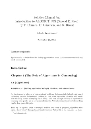
is true, will complete the inductive proof

f (k) ≤ f (n − k − 1) .

2.6

2.4

2.2

2

1.8

f
1.6

1.4

1.2

1
0 1 2 3 4 5 6 7 8 9 10
x

Figure 1: Graphical plot showing the monotonicity of f (x) required for the inductive proof
in Exercise C.1-12.

Further assuming that f has a monotone inverse (to be discussed below) then we can apply
the inverse to this expression to obtain the region of validity for this inequality as

k ≤n−k−1

or k ≤ n−1 . For all the statements above to be valid (and our induction proof to be complete)
2
all one must do now is to show that f (x) has an inverse or equivalently that f (x) is monotonic
over its domain. This could be done with derivatives but rather than that Figure 1 shows a
plot of f (x) showing its monotonic behavior.

Note also from the symmetry relationship possessed by the binomial coefficients, i.e,
n n
=
k n−k
we can extend our result above to all 0 ≤ k ≤ n.

Exercise C.1-13 (Stirling’s approximate for some binomial coefficients)

We desire to show that
2n 22n
= √ (1 + O(1/n))
n πn
using Stirling’s approximation. From the definition of the binomial coefficients we know that
2n (2n)!
= .
n n! n!
Now Stirling’s approximation gives an estimate of n!. Its expression is
√ n n 1
n! = 2πn 1 + θ( ) .
e n

Therefore substituting 2n for n we have an approximation to (2n)! given by

√ 2n
2n 1
(2n)! = 4πn 1 + θ( ) .
e n

We also need an expression for (n!)2 , which is given by
2
n 2n 1
(n!)2 = 2πn 1 + θ( )
e n
n 2n 1
= 2πn 1 + θ( ) .
e n
Thus we have that
√ 2n 2n 1
2n 4πn e
1 + θ( n )
=
n n 2n 1
2πn e
1 + θ( n )
2n 1
1 2n 1 + θ( n )
= √ 1
πn n 1 + θ( n )
22n 1 1
= √ 1 + θ( ) 1 + θ( )
πn n n
2n
2 1
= √ 1 + θ( ) .
πn n
As was to be shown. In deriving this result we have made repeated use of the algebra of
order symbols.

Exercise C.1-14 (the maximum of the entropy function H(λ))

The entropy function is given by

H(λ) = −λ lg(λ) − (1 − λ) lg(1 − λ) .

Remembering the deﬁnition of lg(·) in terms of the natural logarithm ln(·) as

ln(x)
lg(x) =
ln(2)

we have that the derivative of the lg(·) function is given by

lg(x) 1
= .
dx x ln(2)
Using this expression we can take the derivative of the binary entropy function giving
λ (1 − λ)
H ′ (λ) = − lg(λ) − + lg(1 − λ) +
λ ln(2) (1 − λ) ln(2)
= − lg(λ) + lg(1 − λ) .

When we set this equal to zero looking for an extrema we have that
− lg(λ) + lg(1 − λ) = 0
1
which has as its solution λ = 2 . We can check that this point is truly a maximum and not
a minimum by computing the second derivative of H(λ). We have that
1 1
H ′′ (λ) = − − ,
λ ln(2) (1 − λ) ln(2)
1
which is negative when λ = 2
implying a maximum. We also have that
1 1 1
H( ) = + = 1 .
2 2 2

Exercise C.1-15 (moment summing of binomial coeﬃcients)

Consider the binomial expansion learned in high school
n
n n
(x + y) = xk y n−k .
k
k=0

Taking the derivative of this expression with respect to x gives the following
n
n−1 n
n(x + y) = kxk−1 y n−k ,
k
k=0

evaluating at x = y = 1, then gives
n
n
n2n−1 = k,
k
k=0

as was desired to be shown.

Appendix C.2 (Probability)

Exercise C.2-1 (Boole’s inequality)

We begin by decomposing the countable union of sets Ai i.e.
A1 ∪ A2 ∪ A3 . . . ,
into a countable union of disjoint sets Cj . Deﬁne these disjoint sets as
C1 = A1
C2 = A2 A1
C3 = A3 (A1 ∪ A2 )
C4 = A4 (A1 ∪ A2 ∪ A3 )
.
.
.
Cj = Aj (A1 ∪ A2 ∪ A3 ∪ · · · ∪ Aj−1 )

Then by construction
A1 ∪ A2 ∪ A3 · · · = C1 ∪ C2 ∪ C3 · · · ,
and the Cj ’s are disjoint, so that we have

Pr(A1 ∪ A2 ∪ A3 ∪ · · · ) = Pr(C1 ∪ C2 ∪ C3 ∪ · · · ) = Pr(Cj ) .
j

Since Pr(Cj ) ≤ Pr(Aj ), for each j, this sum is bounded above by

Pr(Aj ) ,
j

and Boole’s inequality is proven.

Exercise C.2-2 (more head for professor Rosencrantz)

For this problem we can explicitly enumerate our sample space and then count the number
of occurrences where professor Rosencrantz obtains more heads than professor Guildenstern.
Denoting the a triplet of outcomes from the one coin flip by Rosencrantz and the two coin
flips by Guildenstern as (R, G1 , G2 ), we see that the total sample space for this experiment
is given by
(H, H, H) (H, H, T ) (H, T, H) (H, T, T )
(T, H, H) (T, H, T ) (T, T, H) (T, T, T )
From which the only outcome where professor Rosencrantz obtains more heads than professor
Guildenstern is the sample (H, T, T ). Since this occurs once from eights possible outcomes,
Rosencrantz has a 1/8 probability of winning.

Exercise C.2-3 (drawing three ordered cards)

There are 10 · 9 · 8 = 720 possible ways to draw three cards from ten when the order of the
drawn cards matters. To help motivate how to calculate then number of sorted three card
draws possible, we’ll focus how the number of ordered draws depends on the numerical value
of the first card drawn. For instance, if a ten or a nine is drawn as a first card there are no
possible ways to draw two other cards and have the total set ordered. If an eight is drawn
as the first card, then it is possible to draw a nine for the second and a ten for the third
producing the ordered set (8, 9, 10). Thus if an eight is the first card drawn there is one
possible sorted hand. If a seven is the first card drawn then we can have second and third
draws consisting of (8, 9), (8, 10), or a (9, 10) and have an ordered set of three cards. Once
the seven is drawn we now are looking for the number of ways to draw two sorted cards from
{8, 9, 10}. So if an seven is drawn we have three possible sorted hands. Continuing, if a six
is drawn as the first card we have possible second and third draws of: (7, 8), (7, 9), (7, 10),
(8, 9), (8, 10), or (9, 10) to produce an ordered set. Again we are looking for a way to draw
two sorted cards from a list (this time {7, 8, 9, 10}).

After we draw the first card an important subcalculation is to compute the number of ways
to draw two sorted cards from a list. Assuming we have n ordered items in our list, then
we have n ways to draw the first element and n − 1 ways to draw the second element giving
n(n−1) ways to draw two elements. In this pair of elements one ordering result in a correctly
sorted list (the other will not). Thus half of the above are incorrectly ordered what remains
are
n(n − 1)
N2 (n) =
2
The number of total ways to draw three sorted cards can now be found. If we first draw an
eight we have two cards from which to draw the two remaining ordered cards in N2 (2) ways.
If we instead first drew a seven we have three cards from which to draw the two remaining
ordered cards in N2 (3) ways. If instead we first drew a six then we have four cards from
which to draw two ordered cards in N2 (4) ways. Continuing, if we first draw a one, we have
nine cards from which to draw two ordered cards in N2 (9) ways. Since each of these options
is mutually exclusive the total number of ways to draw three ordered cards is given by
9 9
n(n − 1)
N2 (3) + N2 (4) + N2 (5) + · · · + N2 (9) = N2 (n) = = 120 .
n=2 n=2
2

Finally with this number we can calculate the probability of drawing three ordered cards as
120 1
= .
720 6

Exercise C.2-4 (simulating a biased coin)

Following the hint, since a < b, the quotient a/b is less than one. If we express this number
in binary we will have an (possibly infinite) sequence of zeros and ones. The method to
determine whether to return a biased “heads” (with probability a/b) or a biased “tails”
(with probability (b−a)/b) is best explained with an example. To get a somewhat interesting
binary number, lets assume an example where a = 76 and b = 100, then our ratio a/b is 0.76.
In binary that has a representation given by (see the Mathematica file exercise C 2 4.nb)

0.76 = 0.11000010100011110112

We then begin flipping our unbiased coin. To a “head” result we will associate a one and to
a tail result we shall associate a zero. As long as the outcome of the flipped coin matches
the sequence of ones and zeros in the binary expansion of a/b, we continue flipping. At the
point where the flips of our unbiased coins diverges from the binary sequence of a/b we stop.
If the divergence produces a sequence that is less than the ratio a/b we return this result by
returning a biased “head” result. If the divergence produces a sequence that is greater than
the ratio a/b we return this result by returning a biased “tail” result. Thus we have used
our fair coin to determine where a sequence of flips “falls” relative to the ratio of a/b.

The expected number of coin flips to determine our biased result will be the expected number
of flips required until the flips from the unbiased coin don’t match the sequence of zeros and
ones in the binary expansion of the ratio a/b. If we assume that a success is when our

unbiased coin flip does not match the digit in the binary expansion of a/b. The for each
flip a success can occur with probability p = 1/2 and a failure can occur with probability
q = 1 − p = 1/2, we have that the number of flips n needed before a “success” is a geometric
random variable with parameter p = 1/2. This is that
P {N = n} = q n−1 p .
So that the expected number of flips required for a success is then the expectation of the
geometric random variable and is given by
1
E[N] = = 2,
p
which is certainly O(1).

Exercise C.2-5 (closure of conditional probabilities)

Using the definition of conditional probability given in this section we have that
P {A ∩ B}
P {A|B} = ,
P {B}
so that the requested sum is then given by
¯
P {A ∩ B} P {A ∩ B}
¯
P {A|B} + P {A|B} = +
P {B} P {B}
¯
P {A ∩ B} + P {A ∩ B}
=
P {B}
¯
Now since the events A ∩ B and A ∩ B are mutually exclusive the above equals
¯
P {(A ∩ B) ∪ (A ∩ B)} ¯
P {(A ∪ A) ∩ B} P {B}
= = = 1.
P {B} P {B} P {B}

Exercise C.2-6 (conditioning on a chain of events)

This result follows for the two set case P {A ∩ B} = P {A|B}P {B} by grouping the sequence
of Ai ’s in the appropriate manner. For example by grouping the intersection as
A1 ∩ A2 ∩ · · · ∩ An−1 ∩ An = (A1 ∩ A2 ∩ · · · ∩ An−1 ) ∩ An
we can apply the two set result to obtain
P {A1 ∩ A2 ∩ · · · ∩ An−1 ∩ An } = P {An |A1 ∩ A2 ∩ · · · ∩ An−1 } P {A1 ∩ A2 ∩ · · · ∩ An−1 } .
Continuing now to peal An−1 from the set A1 ∩A2 ∩· · ·∩An−1 we have the second probability
above equal to
P {A1 ∩ A2 ∩ · · · ∩ An−2 ∩ An−1 } = P {An−1|A1 ∩ A2 ∩ · · · ∩ An−2 }P {A1 ∩ A2 ∩ · · · ∩ An−2 } .

Continuing to peal off terms from the back we eventually obtain the requested expression
i.e.

P {A1 ∩ A2 ∩ · · · ∩ An−1 ∩ An } = P {An |A1 ∩ A2 ∩ · · · ∩ An−1 }
× P {An−1 |A1 ∩ A2 ∩ · · · ∩ An−2 }
× P {An−2 |A1 ∩ A2 ∩ · · · ∩ An−3 }
.
.
.
× P {A3 |A1 ∩ A2 }
× P {A2 |A1 }
× P {A1 } .

Exercise C.2-7 (pairwise independence does not imply independence)

Note: As requested by the problem I was not able to find a set of events that are pairwise
independent but such that no subset k > 2 of them are mutually independent. Instead I
found a set of events that are all pairwise independent but that are not mutually independent.
If you know of a solution to the former problem please contact me.

Consider the situation where we have n distinct people in a room. Let Ai,j be the event
that person i and j have the same birthday. We will show that any two of these events are
pairwise independent but the totality of events Ai,j are not mutually independent. That is
we desire to show that the two events Ai,j and Ar,s are independent but the totality of all
n
events are not independent. Now we have that
2

1
P (Ai,j ) = P (Ar,s ) = ,
365
since for the specification of either one persons birthday the probability that the other person
will have that birthday is 1/365. Now we have that

1 1 1
P (Ai,j ∩ Ar,s ) = P (Ai,j |Ar,s )P (Ar,s ) = = .
365 365 3652

This is because P (Ai,j |Ar,s ) = P (Ai,j ) i.e. the fact that persons r and s have the same
birthday has no effect on whether the persons i and j have the same birthday. This is true
even if one of the people in the pairs (i, j) and (r, s) is the same. When we consider the
intersection of all the sets Ai,j , the situation changes. This is because the event ∩(i,j) Ai,j
(where the intersection is over all pairs (i, j)) is the event that every pair of people have the
same birthday, i.e. that everyone considered has the same birthday. This will happen with
probability
n−1
1
,
365

while if the events Ai,j were independent the required probability would be
 
n n(n−1)
1 1
 
2
2
P (Ai,j ) = = .
365 365
(i,j)

n
Since = n − 1, these two results are not equal and the totality of events Ai,j are not
2
independent.

Exercise C.2-8 (conditional but not independence)

Consider the situation where we have to coins. The first coin C1 is biased and has probability
p of landing heads when flipped where p > 1/2. The second coin C2 is fair and has probability
of landing heads 1/2. For our experiment one of the two coins will be selected (uniformly and
at random) and presented to two people who will each flip this coin. We will assume that
the coin that is selected is not known. Let H1 be the event that the first flip lands heads,
and let H2 be the event that the second flip lands heads. We can show that the events H1
and H2 are not independent by computing P (H1 ), P (H2 ), and P (H1 , H2 ) by conditioning
on the coin selected. We have for P (H1 )

P (H1) = P (H1 |C1 )P (C1) + P (H1 |C2 )P (C2)
1 11
= p +
2 22
1 1
= (p + ) ,
2 2
Here C1 is the event that we select the first (biased) coin while C2 is the event we select the
second (unbiased) coin. In the same way we find that
1 1
P (H2 ) = (p + ) ,
2 2
while P (H1, H2 ) is given by

P (H1, H2 ) = P (H1 , H2 |C1 )P (C1) + P (H1 , H2 |C2 )P (C2)
1 11
= p2 +
2 42
1 2 1
= (p + ) .
2 4
The events H1 and H2 will only be independent if P (H1 )P (H2) = P (H1, H2 ) or
2
1 1 1 1
p+ = (p2 + ) .
4 2 2 4

or simplifying this result equality only holds if p = 1/2 which we are assuming is not true.
Now let event E denote the event that we are told that the coin selected and flipped by both

parties is the fair one, i.e. that event C2 happens. Then we have
1 1
P (H1 |E) = and P (H2 |E) =
2 2
1
P (H1 , H2 |E) = .
4
Since in this case we do have P (H1 , H2 |E) = P (H1|E)P (H2|E) we have the required condi-
tional independence. Intuitively, this result makes sense because once we know that the coin
flipped is fair we expect the result of each flip to be independent.

Exercise C.2-9 (the Monte-Hall problem)

Once we have selected a curtain we are two possible situations we might find ourself in. The
first situation A, is where we have selected the curtain with the prize behind it or situation
B where we have not selected the curtain with the prize behind it. The initial probability
of event A is 1/3 and that of event B is 2/3. We will calculate our probability of winning
under the two choices of actions. The first is that we choose not to switch curtains after the
emcee opens a curtain that does not cover the prize. The probability that we win, assuming
the “no change” strategy, can be computed by conditioning on the events A and B above as

P (W ) = P (W |A)P (A) + P (W |B)P (B) .

Under event A and the fact that we don’t switch curtains we have P (W |A) = 1 and
P (W |B) = 0, so we see that P (W ) = 1/3 as would be expected. If we now assume that
we follow the second strategy where by we switch curtains after the emcee revels a curtain
behind which the prize does not sit. In that case P (W |A) = 0 and P (W |B) = 1, since in
this strategy we switch curtains. The the total probability we will is given by
2 2
P (W ) = 0 + 1 · = ,
3 3
since this is greater than the probability we would win under the strategy were we don’t
switch this is the action we should take.

Exercise C.2-10 (a prison delima)

I will argue that X has obtained some information from the guard. Before asking his question
the probability of event X (X is set free) is P (X) = 1/3. If prisoner X is told that Y (or Z
in fact) is to be executed, then to determine what this implies about the event X we need
to compute P (X|¬Y ). Where X, Y , and Z are the events that prisoner X, Y , or Z is to be
set free respectively. Now from Bayes’ rule

P (¬Y |X)P (X)
P (X|¬Y ) = .
P (¬Y )

We have that P (¬Y ) is given by
1 1 2
P (¬Y ) = P (¬Y |X)P (X) + P (¬Y |Y )P (Y ) + P (¬Y |Z)P (Z) = +0+ = .
3 3 3
So the above probability then becomes

1(1/3) 1 1
P (X|¬Y ) = = > .
2/3 2 3

Thus the probability that prisoner X will be set free has increased and prisoner X has
learned from his question.

proof of the cumulative summation formula for E[X] (book notes page 1109)

We have from the definition of the expectation that
∞
E[X] = iP {X = i} .
i=0

expressing this in terms of the the complement of the cumulative distribution function
P {X ≥ i} gives E[X] equal to
∞
i(P {X ≥ i} − P {X ≥ i + 1}) .
i=0

Using the theory of difference equations we write the difference in probabilities above in
terms of the ∆ operator defined on a discrete function f (i) as

∆g(i) ≡ g(i + 1) − g(i) ,

giving
∞
E[X] = − i∆i P {X ≥ i} .
i=0

No using the discrete version of integration by parts (demonstrated here for two discrete
functions f and g) we have
∞ ∞
f (i)∆g(i) = f (i)g(i)|∞
i=1 − ∆f (i)g(i) ,
i=0 i=1

gives for E[X] the following
∞
E[X] = − iP {X ≥ i}|∞
i=1 + P {X ≥ i}
i=1
∞
= P {X ≥ i} .
i=1

1 2 3 4 5 6
1 (2,1) (3,2) (4,3) (5,4) (6,5) (7,6)
2 (2,2) (4,2) (5,3) (6,4) (7,5) (8,6)
3 (4,3) (5,3) (6,3) (7,4) (8,5) (9,6)
4 (5,4) (6,4) (7,4) (8,4) (9,5) (10,6)
5 (6,5) (7,5) (8,5) (9,5) (10,5) (11,6)
6 (7,6) (8,6) (9,6) (10,6) (11,6) (12,6)

Table 1: The possible values for the sum (the ﬁrst number) and the maximum (the second
number) observed when two die are rolled.

which is the desired sum. To see this another way we can explicitly write out the summation
given above and cancel terms as in
∞
E[X] = i(P {X ≥ i} − P {X ≥ i + 1})
i=0
= 0 + P {X ≥ 1} − P {X ≥ 2}
+ 2P {X ≥ 2} − 2P {X ≥ 3}
+ 3P {X ≥ 3} − 3P {X ≥ 4} + . . .
= P {X ≥ 1} + P {X ≥ 2} + P {X ≥ 3} + . . . ,

verifying what was claimed above.

Appendix C.3 (Discrete random variables)

Exercise C.3-1 (expectation of the sum and maximum of two die)

We will begin by computing all possible sums and maximum that can be obtained when we
roll two die. These numbers are computed in table 1, where the row corresponds to the ﬁrst
die and the column corresponds to the second die. Since each roll pairing has a probability
of 1/36 of happening we see that the expectation of the sum S is given by

1 2 3 4 5 6
E[S] = 2 +3 +4 +5 +6 +7
36 36 36 36 36 36
5 4 3 2 1
+ 8 +9 + 10 + 11 + 12
36 36 36 36 36
= 6.8056 .

While the expectation of the maximum M is given by a similar expression

1 3 5 7 9 11
E[M] = 1 +2 +3 +4 +5 +6
36 36 36 36 36 36
= 4.4722 .

Exercise C.3-2 (expectation of the index of the max and min of a random array)

Since the array elements are assumed random the maximum can be at any of the n indices
with probability 1/n. Thus if we define X to be the random variable representing the location
of the maximum of our array we see that the expectation of X is given by
1 1 1
E[X] = 1 +2 + ···+n
n n n
n
1 1 n(n + 1)
= k=
n k=1
n 2
n+1
= .
2
The same is true for the expected location of the minimum.

Exercise C.3-3 (expected cost of playing a carnival game)

Define X to be the random variable denoting the payback from one play of the carnival
game. Then the payback depends on the possible outcomes after the player has guessed a
number. Let E0 be the event that the player’s number does not appear on any die, E1 the
event that the player’s number appears on only one of the three die, E2 the event that the
player’s number appears on only two of the die, and finally E3 the event that the player’s
number appears on all three of the die. The the expected payback is given by
E[X] = −P (E0 ) + P (E1 ) + 2P (E2 ) + 3P (E3 ) .
We now compute the probability of each of the events above. We have
3
5
P (E0 ) = = 0.5787
6
2
1 5
P (E1 ) = 3 = 0.3472
6 6
1 1 5
P (E2 ) = 3 · · = 0.0694
6 6 6
1
P (E3 ) = 3 = 0.0046 .
6
Where the first equation expresses the fact that each individual die will not match the
player’s selected die with probability of 5/6, so the three die will not match the given die
with probability (5/6)3 . The other probabilities are similar. Using these to compute the
expected payoff using the above formula gives
17
E[X] = − = −0.0787 .
216
To verify that these numbers are correct in the Matlab file exercise C 3 3.m, a Monte-Carlo
simulation is developed verifying these values. This function can be run with the command
exercise C 3 3(100000).

Exercise C.3-4 (bounds on the expectation of a maximum)

We have for E[max(X, Y )] computed using the joint density of X and Y that

E[max(X, Y )] = max(x, y)P {X = x, Y = y}
x y

≤ (x + y)P {X = x, Y = y} ,
x y

since X and Y are non-negative. Then using the linearity of the above we have

E[max(X, Y )] ≤ xP {X = x, Y = y} + yP {X = x, Y = y}
x y x y

= xP {X = x} + yP {Y = y}
x y
= E[X] + E[Y ] ,

which is what we were to show.

Exercise C.3-5 (functions of independent variables are independent)

By the independence of X and Y we know that

P {X = x, Y = y} = P {X = x}P {Y = y} .

But by deﬁnition of the random variable X has a realization equal to x then the random
variable f (X) will have a realization equal to f (x). The same statement hold for the random
variable g(Y ) which will have a realization of g(y). Thus the above expression is equal to
(almost notationally)

P {f (X) = f (x), g(Y ) = g(y)} = P {f (X) = f (x)}P {g(Y ) = g(y)}

Deﬁning the random variable F by F = f (X) (an instance of this random variable f ) and
the random variable G = g(Y ) (similarly and instance of this random variable g) the above
shows that
P {F = f, G = g} = P {F = f }P {G = g}
or
P {f (X) = f, g(Y ) = g} = P {f (X) = f }P {g(Y ) = g} ,
showing that f (X) and g(Y ) are independent as requested.

Exercise C.3-6 (Markov’s inequality)

To prove that
E[X]
P {X ≥ t} ≤ ,
t

is equivalent to proving that
E[X] ≥ tP {X ≥ t} .
To prove this first consider the expression for E[X] broken at t i.e.

E[X] = xP {X = x}
x

= xP {X = x} + xP {X = x} .
x<t x≥t

But since X is non-negative we can drop the expression x<t xP {X = x} from the above
and obtain a lower bound. Specifically we have

E[X] ≥ xP {X = x}
x≥t

≥ t P {X = x}
x≥t
= tP {X ≥ t} ,

or the desired result.

Exercise C.3-7 (if X(s) ≥ X ′ (s) then P {X ≥ t} ≥ P {X ′ ≥ t})

Lets begin by defining two sets At and Bt as follows

At = {s ∈ S : X(s) ≥ t}
Bt = {s ∈ S : X ′ (s) ≥ t} .

Then lets consider an element s ∈ Bt . Since s is in Bt we know that X ′ (˜) > t. From the
˜ ˜ s
assumption on X and X ′ we know that X(˜) ≥ X ′ (˜) ≥ t, and s must also be in At . Thus
s s ˜
the set Bt is a subset of the set At . We therefore have that

P {X ≥ t} = P {s} ≥ P {s} = P {X ′ ≥ t} ,
s∈At s∈Bt

and the desired result is obtained.

Exercise C.3-8 (E[X 2 ] > E[X]2 )

From the calculation of the variance of the random variable X we have that

Var(X) = E[(X − E[X])2 ] > 0 ,

since the square in the expectation is always a positive number. Expanding this square we
find that
E[X 2 ] − E[X]2 > 0 .

Which shows on solving for E[X 2 ] that
E[X 2 ] > E[X]2 ,
or that the expectation of the square of the random variable is larger than the square of
the expectation. This make sense because if X where to take on both positive and negative
values in computing E[X]2 the expectation would be decreased by X taking on instances of
both signs. The expression E[X 2 ] would have no such diﬃculty since X 2 is aways positive
regardless of the sign of X.

Exercise C.3-9 (the variance for binary random variables)

Since X takes on only value in {0, 1}, lets assume that
P {X = 0} = 1 − p
P {X = 1} = p .
Then the expectation of X is given by E[X] = 0(1 − p) + 1p = p. Further the expectation
of X 2 is given by E[X 2 ] = 0(1 − p) + 1p = p. Thus the variance of X is given by
Var(X) = E[X 2 ] − E[X]2
= p − p2 = p(1 − p)
= E[X](1 − E[X])
= E[X] E[1 − X] .
Where the transformation 1 − E[X] = E[1 − X] is possible because of the linearity of the
expectation.

Exercise C.3-10 (the variance for aX)

From the suggested equation we have that
Var(aX) = E[(aX)2 ] − E[aX]2
= E[a2 X 2 ] − a2 E[X]2
= a2 (E[X 2 ] − E[X]2 )
= a2 Var(X) ,
by using the linearity property of the expectation.

Appendix C.4 (The geometric and binomial distributions)

an example with the geometric distribution (book notes page 1112)

All the possible outcomes for the sum on two die are given in table 1. There one sees that the
sum of a 7 occurs along the right facing diagonal (elements (6, 1), (5, 5), (4, 3), (3, 4), (2, 5), (1, 6)),

Weatherwax cormen solutions

Recommandé

Recommandé

Contenu connexe

Tendances

Tendances (19)

Similaire à Weatherwax cormen solutions

Similaire à Weatherwax cormen solutions (20)

Dernier

Dernier (20)

Weatherwax cormen solutions