SlideShare une entreprise Scribd logo
1  sur  23
Télécharger pour lire hors ligne
Chapter 4
Differentiation
4.1 Derivatives
Consider the curve shown Figure 4.1. It is clear from intuition that the “slope” changes as we move along the
curve. At P , the slope is very steep whereas at P, the slope is gentle (in this sentence, slope means a piece of
ground going up or down).
P
P
Figure 4.1
In elementary coordinate geometry, readers have learnt the concept “slope of a line”. It is a number which
measures how steep is the line. For a non-vertical line, its slope is given by
y2 − y1
x2 − x1
where (x1, y1) and (x2, y2) are two distinct points on the line and the value is independent of the choice of the
two points.
Figure 4.2
For curves, we shouldn’t say “slope of a curve” because at different points of the curve, the slopes are different.
Instead we should say “slope of a curve at a point”. Below is how we define this concept.
104 Chapter 4. Differentiation
First we have a curve 𝒞 and a point P on the curve. To define the slope of 𝒞 at P, take a point Q on the
curve different from P. The line PQ is called a secant line at P. Its slope, denoted by mPQ, can be found using
the coordinates of P and Q. If we let Q move along the curve, the slope mPQ changes.
𝒞
Q
P
Figure 4.3
Suppose that as Q approaches P, the number mPQ approaches a fixed value. This value, denoted by m𝒞,P or
simply mP if the curve is understood, is called the slope of 𝒞 at P; and the line with slope mP and passing
through P is called the tangent line to the curve 𝒞 at P.
Remark The number m𝒞,P (if exist) is the unique real number satisfying
(∗) mPQ is arbitrarily close to m𝒞,P if Q belonging to 𝒞 is sufficiently close to (but different from) P.
In view of the concept “limit of a function at a point” and the notation lim
x→a
f(x), we may write
lim
Q→P
along 𝒞
mPQ = m𝒞,P
to mean that (∗) holds. Below, we will discuss how to find lim
Q→P
along 𝒞
mPQ by rewriting it as the limit of a difference
quotient.
Formula for Slope Suppose 𝒞 is given by y = f(x), where f is a function; and P(x0, f(x0)) is a point on 𝒞.
For any point Q on 𝒞 with Q P, its x-coordinate can be written as x0 + h where h 0 (if h > 0, Q is on the
right of P; if h < 0, Q is on the left of P). Thus, Q can be written as (x0 + h, f(x0 + h)). The slope mPQ of the
secant line PQ is
mPQ =
f(x0 + h) − f(x0)
(x0 + h) − x0
=
f(x0 + h) − f(x0)
h
Note that as Q approaches P, the number h approaches 0. From these, we see that the slope of 𝒞 at P (denoted
by mP) is
mP = lim
h→0
f(x0 + h) − f(x0)
h
(4.1.1)
provided that the limit exists.
Remark The limit in (4.1.1) is a two-sided limit. This is because Q can approach P from the left or from the
right and so h can approach 0 from the left or from the right.
4.1. Derivatives 105
Example Find the slope of the curve given by y = x2 at the point P(3, 9).
Solution Put f(x) = x2. By (4.1.1), the required slope (denoted by mP) is
mP = lim
h→0
f(3 + h) − f(3)
h
= lim
h→0
(3 + h)2 − 32
h
= lim
h→0
(9 + 6h + h2) − 9
h
= lim
h→0
6h + h2
h
= lim
h→0
(6 + h)
= 6.
-3-2-1 1 2 3
2
4
6
8
10
12
14
Figure 4.4
Definition Let x0 be a real number and let f be a function defined on an open interval containing x0. Suppose
the limit in (4.1.1) exists. Then we say that f is differentiable at x0.
Convention Open intervals will be denoted by (a, b) including the cases where a = −∞ and/or b = ∞, unless
otherwise stated. Thus (a, b) can be any one of the following:
• (a, b) where a, b ∈ R and a < b;
• (−∞, b) where a = −∞ and b ∈ R;
• (a, ∞) where a ∈ R and b = ∞;
• (−∞, ∞) where a = −∞ and b = ∞.
Remark
• The condition “f is a function defined on an open interval containing x0” means that there is an open
interval (a, b) such that (a, b) ⊆ dom (f) and x0 ∈ (a, b). Hence, f is defined on the left-side and right-side
of x0 as well as at x0. The expression
f(x0 + h) − f(x0)
h
in the limit in (4.1.1), considered as a function of h,
is defined on the left-side and the right-side of 0 but is undefined at 0.
• “f is differentiable at x0” means that the slope of the curve 𝒞 at P exists, where 𝒞 is given by y = f(x)
and P is the point on 𝒞 whose x-coordinate is x0.
• There is an alternative way to describe the limit in (4.1.1). Putting x = x0 + h, we have x − x0 = h. Note
that as h approaches to 0, x approaches to x0. Hence we have
lim
h→0
f(x0 + h) − f(x0)
h
= lim
x→x0
f(x) − f(x0)
x − x0
.
Theorem 4.1.1 Let x0 be a real number and let f be a function defined on an open interval containing x0.
Suppose f is differentiable at x0. Then f is continuous at x0.
106 Chapter 4. Differentiation
Proof Since f is differentiable at x0, by definition, lim
x→x0
f(x) − f(x0)
x − x0
exists (a real number). Hence we have
lim
x→x0
f(x) − f(x0) = lim
x→x0
f(x) − f(x0)
x − x0
· (x − x0)
= lim
x→x0
f(x) − f(x0)
x − x0
· lim
x→x0
(x − x0) Limit Rule (La5)
= lim
x→x0
f(x) − f(x0)
x − x0
· (x0 − x0) Theorem 3.5.1
= lim
x→x0
f(x) − f(x0)
x − x0
· 0
= 0.
Therefore, we get
lim
x→x0
f(x) = lim
x→x0
f(x) − f(x0) + f(x0)
= lim
x→x0
f(x) − f(x0) + lim
x→x0
f(x0) Limit Rule (La4)
= 0 + f(x0) From above and Limit Rule (La1)
= f(x0).
That is, f is continuous at x0.
The following example illustrates that converse of Theorem 4.1.1 is not true.
Example Let f(x) = |x|. The domain of f is R.
The function f is continuous at 0. This is because
• lim
x→0−
f(x) = lim
x→0−
(−x) = 0;
• lim
x→0+
f(x) = lim
x→0+
x = 0,
and so lim
x→0
f(x) = 0 = f(0).
-2 -1 1 2
1
2
Figure 4.5
However, f is not differentiable at 0. This is because lim
h→0
f(0 + h) − f(0)
h
does not exist as the left-side and
right-side limits are unequal:
lim
h→0+
f(0 + h) − f(0)
h
= lim
h→0+
h − 0
h
= lim
h→0+
1
= 1
and lim
h→0−
f(0 + h) − f(0)
h
= lim
h→0−
−h − 0
h
= lim
h→0−
−1
= −1.
Definition Let f be a function.
(1) Suppose that f is differentiable at every point belonging to an open interval (a, b). Then we say that f is
differentiable on (a, b).
4.1. Derivatives 107
(2) Suppose that f is differentiable at every point belonging to its domain. Then we say that f is a differen-
tiable function.
Remark If f is a differentiable function, then its domain can be written as a union of open intervals.
Example Let f(x) = |x|. In a previous example, we have seen that f is not differentiable at 0. Thus f is not a
differentiable function. Below we will show that f is differentiable at every x0 0. Thus, f is differentiable on
(0, ∞) as well as on (−∞, 0).
(x0 > 0) In this case, if h is a small enough real number, then x0 + h > 0 and so we have
f(x0 + h) − f(x0) = |x0 + h| − |x0|
= (x0 + h) − x0 = h,
which yields
lim
h→0
f(x0 + h) − f(x0)
h
= lim
h→0
h
h
= lim
h→0
1 = 1.
(x0 < 0) In this case, if h is a small enough real number, then x0 + h < 0 and so we have
f(x0 + h) − f(x0) = |x0 + h| − |x0|
= −(x0 + h) − (−x0) = −h,
which yields
lim
h→0
f(x0 + h) − f(x0)
h
= lim
h→0
−h
h
= lim
h→0
−1 = −1.
A function f is differentiable means that for every x ∈ dom (f), the limit of the difference quotient
lim
h→0
f(x + h) − f(x)
h
exists; the limit is a real number and its value depends on x. In this way, we get a func-
tion, called the derivative of f and denoted by f , from dom (f) to R.
The graph of f is a curve. The assumption that f is a
differentiable function implies that at every point on the
curve, the slope exists; at the point whose x-coordinate is
x0, the slope is f (x0). Thus f can be considered as slope
function.
y = f(x)
(x0, f(x0))
slope = f (x0)
(x1, f(x1))
slope = f (x1)
Figure 4.6
More generally, if f is differentiable only at some points in its domain, we can still define the derivative of
f on a smaller set.
Definition Let f be a function that is differentiable at some points belonging in its domain. Then the derivative
of f, denoted by f , is the function (from a subset of dom (f) into R) given by
f (x) = lim
h→0
f(x + h) − f(x)
h
,
108 Chapter 4. Differentiation
where the domain of f is x ∈ dom ( f) : lim
h→0
f(x + h) − f(x)
h
exists .
Example Let f(x) = |x|. Using results in a previous example, we see that
f (x) =



1 if x > 0,
−1 if x < 0,
where dom (f ) = {x ∈ R : x 0}.
Example Let f(x) = x2. Find the derivative of f.
Explanation To find the derivative of f means to find the domain of f and find a formula for f (x).
Solution By definition, we have
f (x) = lim
h→0
f(x + h) − f(x)
h
= lim
h→0
(x + h)2 − x2
h
= lim
h→0
(x2 + 2xh + h2) − x2
h
= lim
h→0
2xh + h2
h
= lim
h→0
(2x + h)
= 2x.
The domain of f is R.
Remark The logic in the above solution is as follows:
(1) First we find that lim
h→0
f(x + h) − f(x)
h
= 2x for all x ∈ R.
(2) From (1), we see that the domain of f is R and f (x) = 2x for all x ∈ R.
Example Let f(x) = x3. Find f (x).
Solution By definition, we have
f (x) = lim
h→0
f(x + h) − f(x)
h
= lim
h→0
(x + h)3 − x3
h
= lim
h→0
(x3 + 3x2h + 3xh2 + h3) − x3
h
= lim
h→0
3x2h + 3xh2 + h3
h
= lim
h→0
(3x2 + 3xh + h2)
= 3x2.
4.1. Derivatives 109
Remark The domain of f is R.
Terminology The process of finding derivatives is called differentiation.
In a previous example to find the slope of the parabola y = f(x) = x2 at the point (3, 9), we use definition to
find f (3). In fact, if we know that f (x) = 2x, then by direct substitution, we get f (3) = 6. In the next section,
we will discuss how to find f (x) using rules for differentiation.
Terminology f (x0) is called the derivative of f at x0.
To represent a function f, we sometimes write y or f(x). Similarly, the derivative of a function can be
represented in many ways.
Notation
• To denote the derivative of a function f, we have the following notations.
f , y ,
dy
dx
, Df, Dy, f (x) and
d
dx
f(x).
• To denote the derivative of f at x0, we have the following notations.
f (x0), y (x0),
dy
dx x=x0
, Df(x0) and Dy(x0).
Some readers may wonder why we have the notation as well as the
d
dx
notation. Calculus was “invented” by Newton and Leibniz independently
in the late 17th century. Newton used ˙x whereas Leibniz used
dx
dt
to denote
the derivative of x with respect to t (time). The notation y is simple whereas
dy
dx
reminds us that it is defined as a limit of difference quotient:
dy
dx
= lim
∆x→0
∆y
∆x
where ∆x = h = (x + h) − x and ∆y = f(x + h) − f(x) are changes in x and
y respectively.
∆y
∆x
Figure 4.7
Caution
dy
dx
is not a fraction.
•
dy
dx
is f or f (x); it is a function or an expression in x. It can be written as
d
dx
y also. The notation
d
dx
can be considered as an operation; to find
dy
dx
means to perform the differentiation operation on y. Some
authors use the notation Dy instead, where D stands for the differentiation operator (some authors use
Dxy to emphasize that the variable is x).
• Although we can define dy and dx (called differentials),
dy
dx
does not mean “divide dy by dx”. In Chap-
ter 10, we will describe differentials briefly (the purpose is to introduce the substitution method for
integration).
110 Chapter 4. Differentiation
Using
d
dx
notation, the results obtained in the last two examples can be written as
d
dx
x2 = 2x
d
dx
x3 = 3x2.
In Exercise 3.5, Question 2(c) and (d), in terms of the
d
dx
notation, the answers can be written as
d
dx
x−1 = −x−2
d
dx
x
1
2 =
1
2
x−1
2 .
These are particular cases of a general result, called the power rule which will be discussed in Section 4.2.
Rate of Change
• The slope of a line is the rate of change of y with respect to x. The slope of a curve y = f(x) at a point
P x0, f(x0) is the limit of the slopes of the secant lines through P, so it is the rate of change of y with
respect to x at P. That is, f (x0) or
dy
dx x=x0
is the rate of change of y with respect to x when x = x0.
• If x = t is time and y = s(t) is the displacement function of a moving object then s (t0) or
ds
dt t=t0
is the
rate of change of displacement with respect to time when t = t0, that is, the (instantaneous) velocity at
t = t0. In the Introduction of Chapter 3, we consider the velocity of an object at time t = 2, where the
displacement function is s(t) = t2. Using differentiation, the velocity at t = 2 can be found easily:
s (2) =
d
dt
t2
t=2
= 2t t=2
= 4.
Remark The notation 2t t=2
means substitute t = 2 into the expression 2t. More generally, the notation
f(x) x=x0
means f(x0).
Exercise 4.1
1. For each of the following f, use definition to find f (x).
(a) f(x) = 2x2 + 1 (b) f(x) = x3 − 3x
(c) f(x) = x4 (d) f(x) =
1
x2
4.2 Rules for Differentiation
Derivative of Constant The derivative of a constant function is 0 (the zero function), that is
d
dx
c = 0,
where c is a constant.
4.2. Rules for Differentiation 111
Explanation In the above formula, we use c to denote the constant function f given by f(x) = c. The domain
of f is R. The result means that f is differentiable on R and that f (x) = 0 for all x ∈ R.
Proof Let f : R −→ R be the function given by f(x) = c for x ∈ R. By definition, we get
f (x) = lim
h→0
f(x + h) − f(x)
h
= lim
h→0
c − c
h
= lim
h→0
0
h
= lim
h→0
0
= 0
Geometric meaning The graph of the constant function c is the horizontal line given by y = c. At every point
on the line, the slope is 0.
Derivative of Identity Function The derivative of the identity function is the constant function 1, that is
d
dx
x = 1.
Explanation In the above formula, we use x to denote the identity function, that is, the function f given by
f(x) = x. The domain of f is R. The result means that f is differentiable on R and f (x) = 1 for all x ∈ R.
Proof Let f : R −→ R be the function given by f(x) = x for x ∈ R. By definition, we get
f (x) = lim
h→0
f(x + h) − f(x)
h
= lim
h→0
x + h − x
h
= lim
h→0
h
h
= lim
h→0
1
= 1
Geometric meaning The graph of the identity function is the line given by y = x. At every point on the line, the
slope is 1.
Power Rule for Differentiation (positive integer version) Let n be a positive integer. Then the power function
xn is differentiable on R and we have
d
dx
xn
= nxn−1
.
Explanation In the above formula, we use xn to denote the n-th power function, that is, the function f given
by f(x) = xn. The domain of f is R. The result means that f is differentiable on R and f (x) = nxn−1 for all
112 Chapter 4. Differentiation
x ∈ R. When n = 1, the formula becomes
d
dx
x = 1x0. In the expression on the right side, x0 is understood to
be the constant function 1 and so the formula reduces to
d
dx
x = 1 which is the rule for derivative of the identity
function. To prove that the result is true for all positive integers n, we can use mathematical induction. For base
step, we know that the result is true when n = 1. For the induction step, we can apply product rule (will be
discussed later). Below we will give alternative proofs for the power rule (positive integer version).
Proof Let f : R −→ R be the function given by f(x) = xn for x ∈ R. By definition, we get
f (x) = lim
h→0
f(x + h) − f(x)
h
= lim
h→0
(x + h)n − xn
h
.
To find the limit, we “simplify” the numerator to obtain a factor h and then cancel it with the factor h in the
denominator. For this, we can use:
• a factorization formula an − bn = (a − b)(an−1 + an−2b + · · · + abn−2 + bn−1)
• the Binomial Theorem (a + b)n = an + n
1 an−1b + n
2 an−2b2 + · · · + n
n−2 a2bn−2 + n
n−1 abn−1 + bn
where n
1 = n and n
2 =
n(n − 1)
2
and n
3 =
n(n − 1)(n − 2)
3 · 2
etc. are the binomial coefficients (see Binomial
Theorem in the appendix). However, in the proof below, we only need to know the coefficient n
1 = n;
the other coefficients are not important.
(Method 1) By the factorization formula, we get
(x + h)n − xn = (x + h − x) (x + h)n−1 + (x + h)n−2x + · · · + (x + h)xn−2 + xn−1
= h (x + h)n−1 + (x + h)n−2x + · · · + (x + h)xn−2 + xn−1
Therefore, f (x) = lim
h→0
(x + h)n−1 + (x + h)n−2x + · · · + (x + h)xn−2 + xn−1
= (x + 0)n−1 + (x + 0)n−2 · x + · · · + (x + 0) · xn−2 + xn−1 Theorem 3.5.1
= xn−1
+ xn−1
+ · · · + xn−1
+ xn−1
n terms
= nxn−1
(Method 2) From the Binomial Theorem, we get
(x + h)n − xn = xn + n
1 xn−1h + n
2 xn−2h2 + · · · + n
n−2 x2hn−2 + n
n−1 xhn−1 + hn − xn
= n
1 xn−1h + n
2 xn−2h2 + · · · + n
n−2 x2hn−2 + n
n−1 xhn−1 + hn
= h nxn−1 + n
2 xn−2h + · · · + n
n−2 x2hn−3 + n
n−1 xhn−2 + hn−1 because n
1 = n
Therefore, f (x) = lim
h→0
nxn−1 + n
2 xn−2h + · · · + n
n−2 x2hn−3 + n
n−1 xhn−2 + hn−1
= nxn−1 + n
2 xn−2 · 0 + · · · + n
n−2 x2 · 0 + n
n−1 x · 0 + 0 Theorem 3.5.1
= nxn−1.
4.2. Rules for Differentiation 113
Example Let y = x123. Find
dy
dx
.
Explanation The notation y = x123 represents a power function. To find
dy
dx
means to find the derivative of the
function.
Solution
dy
dx
=
d
dx
x123
= 123x123−1 Power Rule
= 123x122
Caution In the above solution, the first step is “substitution”. It can also be written as
dx123
dx
. It is wrong to write
dy
dx
x123 which means
dy
dx
multiplied by x123. The notation
d
dx
x123 is the derivative of the power function x123. If
we consider
d
dx
as an operator,
d
dx
x123 means “perform the differentiation operation on the function x123”.
Remark
• In the power rule, if we put n = 0, the left side is
d
dx
x0 and right side is 0x−1. The function x0 is understood
to be the constant function 1. Thus
d
dx
x0 = 0 by the rule for derivative of constant. The domain of the
function x−1 is R  {0}. Therefore, 0x−1 is the function whose domain is R  {0} and is always equal to 0.
If we extend the domain to R and treat 0x−1 as the constant function 0, then the power rule is true when
n = 0.
• Later in this section, we will show that the power rule is also true for negative integers n using the quotient
rule (in fact, it is true for all real numbers n; the result will be called the general power rule).
• In Chapter 6, we will discuss integration which is the reverse process of differentiation. There is a result
called the power rule for integration. However, in this chapter, “power rule” always means “power rule
for differentiation”.
Constant Multiple Rule for Differentiation Let f be a function and let k be a constant. Suppose that f is
differentiable. Then the function k f is also differentiable. Moreover, we have
d
dx
(k f)(x) = k ·
d
dx
f(x).
Explanation The function k f is defined by (k f)(x) = k · f(x) for x ∈ dom (f). The result means that if f (x)
exists for all x ∈ dom ( f), then (k f) (x) = k · f (x) for all x ∈ dom ( f), that is, (k f) = k · f .
Proof By definition, we have
(k f) (x) = lim
h→0
(k f)(x + h) − (k f)(x)
h
= lim
h→0
k · f(x + h) − k · f(x)
h
Definition of k f
= lim
h→0
k ·
f(x + h) − f(x)
h
= k · lim
h→0
f(x + h) − f(x)
h
Limit Rule (La5s)
= k · f (x)
114 Chapter 4. Differentiation
Remark There is a pointwise version of the constant multiple rule: the result remains valid if differentiable
function is replaced by differentiable at a point.
Let f be a function and let k be a constant. Suppose that f is differentiable at x0. Then the function k f is
also differentiable at x0. Moreover, we have (k f) (x0) = k · f (x0)
There are also pointwise versions for the sum rule, product rule and quotient rule which will be discussed
later. Readers can formulate the results themselves.
Example Let y = 3x4. Find
dy
dx
.
Solution
dy
dx
=
d
dx
3x4
= 3 ·
d
dx
x4 Constant Multiple Rule
= 3 · (4x4−1) Power Rule
= 12x3
Sum Rule for Differentiation (Term by Term Differentiation) Let f and g be functions with the same domain.
Suppose that f and g are differentiable. Then the function f + g is also differentiable. Moreover, we have
d
dx
( f + g)(x) =
d
dx
f(x) +
d
dx
g(x).
Explanation The function f + g is defined by (f + g)(x) = f(x) + g(x) for x belonging to the common domain
A of f and g. The result means that if f (x) and g (x) exist for all x ∈ A, then (f + g) (x) = f (x) + g (x) for all
x ∈ A, that is, (f + g) = f + g .
Proof By definition, we have
( f + g) (x) = lim
h→0
( f + g)(x + h) − ( f + g)(x)
h
= lim
h→0
f(x + h) + g(x + h) − f(x) + g(x)
h
Definition of f + g
= lim
h→0
f(x + h) − f(x) + g(x + h) − g(x)
h
= lim
h→0
f(x + h) − f(x)
h
+
g(x + h) − g(x)
h
= lim
h→0
f(x + h) − f(x)
h
+ lim
h→0
g(x + h) − g(x)
h
Limit Rule (La4)
= f (x) + g (x)
Remark
• If the domains of f and g are not the same but their intersection is nonempty, we define f + g to be the
function with domain dom (f) ∩ dom (g) given by (f + g)(x) = f(x) + g(x). The following is a more
general version of the sum rule:
4.2. Rules for Differentiation 115
Let f and g be functions. Suppose that f and g are differentiable on an open interval (a, b). Then the
function f + g is also differentiable on (a, b). Moreover, on the interval (a, b), we have
d
dx
(f + g)(x) =
d
dx
f(x) +
d
dx
g(x).
There are also more general versions for the product rule and quotient rule. Readers can formulate the
results themselves.
• The result is also true for difference of two functions, that is,
d
dx
(f − g)(x) =
d
dx
f(x) −
d
dx
g(x).
The result for difference can be proved similar to that for sum. Alternatively, it can be proved from the
sum rule together with the constant multiple rule:
( f − g) (x) = ( f + (−1)g) (x)
= f (x) + (−1)g (x) Sum Rule
= f (x) + (−1) · g (x) Constant Multiple Rule
= f (x) − g (x).
• Term by Term Differentiation can be applied to sum and difference of finitely many terms.
Example Let y = x2 + 3. Find
dy
dx
.
Solution
dy
dx
=
d
dx
(x2 + 3)
=
d
dx
x2 +
d
dx
3 Term by Term Differentiation
= 2x + 0 Power Rule and Derivative of Constant
= 2x
Example Let f(x) = x5 − 6x7. Find f (x).
Explanation This question is similar to the last one. If we put y = f(x), then f (x) =
dy
dx
. Below, we use the
notation
d
dx
to perform differentiation.
Solution f (x) =
d
dx
(x5 − 6x7)
=
d
dx
x5 −
d
dx
6x7 Term by Term Differentiation
= 5x4 − 6 ·
d
dx
x7 Power Rule and Constant Multiple Rule
= 5x4 − 6 · (7x6) Power Rule
= 5x4 − 42x6
116 Chapter 4. Differentiation
The last two examples illustrate that polynomials can be differentiated term by term.
Derivative of Polynomial Let y = anxn + an−1xn−1 + · · · + a2x2 + a1x + a0 be a polynomial. Then we have
dy
dx
= nanxn−1
+ (n − 1)an−1xn−2
+ · · · + 2a2x + a1.
Proof
dy
dx
=
d
dx
anxn + an−1xn−1 + · · · + a2x2 + a1x + a0
=
d
dx
anxn +
d
dx
an−1xn−1 + · · · +
d
dx
a2x2 +
d
dx
a1x +
d
dx
a0 Term by Term Differentiation
= an
d
dx
xn + an−1
d
dx
xn−1 + · · · + a2
d
dx
x2 + a1
d
dx
x + 0
Constant Multiple Rule and
Derivative of Constant
= annxn−1 + an−1(n − 1)xn−2 + · · · + a2 · (2x) + a1 · 1 Power Rule
Example Let f(x) = 2x (x2 − 5x + 7). Find the derivative of f at 2.
Explanation The question is to find f (2). We can find f (x) using one of the following two ways:
• product rule (will be discussed later);
• expand the expression to get a polynomial.
Then putting x = 2, we get the answer. Below we use the second method to find f (x).
Solution f (x) =
d
dx
2x (x2 − 5x + 7)
=
d
dx
2x3 − 10x2 + 14x
= 2 · (3x2) − 10 · (2x) + 14 · 1 Derivative of Polynomial
= 6x2 − 20x + 14
The derivative of f at 2 is f (2) = 6(22) − 20(2) + 14
= −2
Product Rule Let f and g be functions with the same domain. Suppose that f and g are differentiable. Then
the function fg is also differentiable. Moreover, we have
d
dx
(fg)(x) = g(x) ·
d
dx
f(x) + f(x) ·
d
dx
g(x).
Explanation The function fg is defined by (fg)(x) = f(x) · g(x) for x belonging to the common domain A of f
and g. The result means that if f (x) and g (x) exist for all x ∈ A, then (fg) (x) = g(x)f (x) + f(x)g (x) for all
x ∈ A, that is, (fg) = gf + fg .
Proof By definition, we have
(fg) (x) = lim
h→0
(fg)(x + h) − (fg)(x)
h
= lim
h→0
f(x + h)g(x + h) − f(x)g(x)
h
Definition of fg
4.2. Rules for Differentiation 117
To find the limit, we use the following technique: “subtract and add” f(x + h)g(x) in the numerator.
( fg) (x) = lim
h→0
f(x + h)g(x + h) − f(x + h)g(x) + f(x + h)g(x) − f(x)g(x)
h
= lim
h→0
f(x + h)g(x + h) − f(x + h)g(x)
h
+
f(x + h)g(x) − f(x)g(x)
h
= lim
h→0
f(x + h) ·
g(x + h) − g(x)
h
+ lim
h→0
g(x) ·
f(x + h) − f(x)
h
Limit Rule (La4)
= lim
h→0
f(x + h) · lim
h→0
g(x + h) − g(x)
h
+ lim
h→0
g(x) · lim
h→0
f(x + h) − f(x)
h
Limit Rule (La5)
= f(x)g (x) + g(x) f (x) Theorem 4.1.1 &
Limit Rule (La1)
In the last step, the first limit is found by substitution because f is continuous; the third limit is g(x) because
considered as a function of h, g(x) is a constant.
Example Let y = (x + 1)(x2 + 3). Find
dy
dx
.
Explanation The expression defining y is a product of two functions. So we can apply the product rule. Alter-
natively, we can expand the expression to get a polynomial and then differentiate term by term.
Solution 1
dy
dx
=
d
dx
(x + 1)(x2 + 3)
= (x2 + 3) ·
d
dx
(x + 1) + (x + 1) ·
d
dx
(x2 + 3) Product Rule
= (x2 + 3) · (1 + 0) + (x + 1) · (2x + 0) Derivative of Polynomial
= 3x2 + 2x + 3
Solution 2
dy
dx
=
d
dx
(x + 1)(x2 + 3)
=
d
dx
(x3 + x2 + 3x + 3)
= 3x2 + 2x + 3 Derivative of Polynomial
Quotient Rule Let f and g be functions with the same domain. Suppose that f and g are differentiable and that
g has no zero in its domain. Then the function
f
g
is also differentiable. Moreover, we have,
d
dx
f
g
(x) =
g(x) ·
d
dx
f(x) − f(x) ·
d
dx
g(x)
g(x) 2
.
Explanation The condition “g has no zero in its domain” means that g(x) 0 for all x ∈ dom (g). The function
f
g
is defined by
f
g
(x) =
f(x)
g(x)
for x ∈ A, where A is the common domain of f and g. The result means that if
f (x) and g (x) exist for all x ∈ A, then
f
g
(x) =
g(x) f (x) − f(x)g (x)
g(x)2
for all x ∈ A, that is,
f
g
=
g f − fg
g2
.
118 Chapter 4. Differentiation
Proof The proof is similar to that for the product rule.
Example Let y =
x2 + 3x − 4
2x + 1
. Find
dy
dx
.
Solution
dy
dx
=
d
dx
x2 + 3x − 4
2x + 1
=
(2x + 1) ·
d
dx
(x2 + 3x − 4) − (x2 + 3x − 4) ·
d
dx
(2x + 1)
(2x + 1)2
Quotient Rule
=
(2x + 1)(2x + 3) − (x2 + 3x − 4)(2)
(2x + 1)2
Derivative of Polynomial
=
(4x2 + 8x + 3) − (2x2 + 6x − 8)
(2x + 1)2
=
2x2 + 2x + 11
(2x + 1)2
Power Rule for Differentiation (negative integer version) Let n be a negative integer. Then the power func-
tion xn is differentiable on R  {0} and we have
d
dx
xn
= nxn−1
.
Explanation Since n is a negative integer, it can be written as −m where m is a positive integer. The function
xn = x−m =
1
xm
is defined for all x 0, that is, the domain of xn is R  {0}.
Proof Let f : R  {0} −→ R be the function given by f(x) = x−m, where m = −n. By definition, we have
f (x) =
d
dx
1
xm
=
xm ·
d
dx
1 − 1 ·
d
dx
xm
(xm)2
Quotient Rule
=
xm · 0 − 1 · mxm−1
x2m
Derivative of Constant &
Power Rule (positive integer version)
= −mx(m−1)−2m
= −mx−m−1
= nxn−1
Example Find an equation for the tangent line to the curve y =
3x2
− 1
x
at the point (1, 2).
Explanation The curve is given by y = f(x) where f(x) =
3x2
− 1
x
. Since f(1) = 2, the point (1, 2) lies on the
curve. To find an equation for the tangent line, we have to find the slope at the point (and then use point-slope
form). The slope at the point (1, 2) is f (1). We can use rules for differentiation to find f (x) and then substitute
x = 1 to get f (1).
Solution To find
dy
dx
, we can use quotient rule or term by term differentiation.
4.2. Rules for Differentiation 119
(Method 1)
dy
dx
=
d
dx
3x2 − 1
x
=
x ·
d
dx
(3x2 − 1) − (3x2 − 1) ·
d
dx
x
x2
Quotient Rule
=
x · 3 · (2x) − (3x2 − 1) · 1
x2
Derivative of Polynomial
=
3x2 + 1
x2
(Method 2)
dy
dx
=
d
dx
(3x2 − 1)x−1
=
d
dx
(3x − x−1)
=
d
dx
3x −
d
dx
x−1 Term by Term Differentiation
= 3 − (−1)x−2 Derivative of Polynomial & Power Rule
= 3 +
1
x2
.
The slope of the tangent line at the point (1, 2) is
dy
dx x=1
= 3 +
1
1
= 4.
Equation for the tangent line: y − 2 = 4(x − 1) (point-slope form)
4x − y − 2 = 0 (general linear form)
The next result is a special case of the general power rule. Since the square root function appears often in
applied problems and the proof is not difficult, we give the result here.
Derivative of the Square Root Function The derivative of the square root function
√
x is
1
2
√
x
, that is,
d
dx
√
x =
1
2
√
x
.
Explanation The domain of the square root function is [0, ∞). Since the function is undefined on the left-side
of 0, we can only consider differentiability of the function on (0, ∞). The result means that f (x) =
1
2
√
x
for all
x ∈ (0, ∞) where f(x) =
√
x.
Proof Let f : [0, ∞) −→ R be the function given by f(x) =
√
x. For every x > 0, note that if h is a small
enough real number, then x + h ∈ dom (f) and hence if h is a small enough non-zero real number, we have
f(x + h) − f(x)
h
=
√
x + h −
√
x
h
=
√
x + h −
√
x
√
x + h +
√
x
h
√
x + h +
√
x
=
(x + h) − x
h
√
x + h +
√
x
=
h
h
√
x + h +
√
x
=
1
√
x + h +
√
x
120 Chapter 4. Differentiation
which, by definition, implies that
f (x) = lim
h→0
1
√
x + h +
√
x
=
1
lim
h→0
√
x + h +
√
x
Limit Rule (La6)
=
1
lim
h→0
√
x + h + lim
h→0
√
x
Limit Rule (La4)
=
1
√
x + 0 +
√
x
By continuity &
Limit Rule (La1)
=
1
2
√
x
In the second last step, the first limit is found by substitution because the square root function is continuous;
the second limit is the limit of a constant.
Example Let y =
√
x (x + 1). Find
dy
dx
.
Solution
dy
dx
=
d
dx
√
x (x + 1)
= (x + 1) ·
d
dx
√
x +
√
x ·
d
dx
(x + 1) Product Rule
= (x + 1) ·
1
2
√
x
+
√
x · 1 Derivative of Square Root Function
& Derivative of Polynomial
=
√
x
2
+
1
2
√
x
+
√
x
=
3
√
x
2
+
1
2
√
x
Remark If we expand the expression defining y, we get x
3
2 + x
1
2 . The derivative can be found if we know the
derivative of x
3
2 .
Power Rule for Differentiation (n + 1
2
version) Let n be an integer. Then the function xn+ 1
2 is differentiable
on (0, ∞) and we have
d
dx
xn+ 1
2 = n +
1
2
xn− 1
2 .
Explanation Denoting the function by f, if n = 0, then f is the square root function; if n is positive, then the
domain of f is [0, ∞); if n is negative, then the domain of f is (0, ∞). Putting r = n +
1
2
, then we have f(x) = xr
and the result means that f (x) = rxr−1 for all x > 0. This result has the same form as the power rule and it will
be referred to as the power rule.
Remark There is a more general result called the General Power Rule (see Chapter 9).
Proof Let f be the function given by f(x) = xn+1
2 . Note that f(x) = xn ·
√
x and so by the Product Rule and the
4.2. Rules for Differentiation 121
Rule for Derivative of the Square Root Function, the function f is differentiable on (0, ∞) and we have
f (x) =
d
dx
xn ·
√
x
=
√
x ·
d
dx
xn + xn ·
d
dx
√
x Product Rule
=
√
x · nxn−1 + xn ·
1
2
√
x
Power Rule &
Derivative Square Root Function
= nxn−1
2 +
1
2
xn−1
2
= n +
1
2
xn− 1
2
Below, we redo the preceding example using the n +
1
2
version of the power rule.
Example Let y =
√
x (x + 1). Find
dy
dx
.
Solution
dy
dx
=
d
dx
x
1
2 (x + 1)
=
d
dx
x
3
2 + x
1
2
=
d
dx
x
3
2 +
d
dx
x
1
2 Term by Term Differentiation
=
3
2
x
3
2 −1 +
1
2
x
1
2 −1 Power Rule
=
3
2
x
1
2 +
1
2
x−1
2
Example Let y =
2x2 − 3
√
x
. Find
dy
dx
.
Solution 1
dy
dx
=
d
dx
2x2 − 3
√
x
=
√
x ·
d
dx
(2x2 − 3) − (2x2 − 3) ·
d
dx
√
x
(
√
x)2
Quotient Rule
=
√
x · 2 · (2x) − (2x2 − 3) ·
1
2
√
x
x
Derivative of Polynomial &
Derivative of Square Root Function
=
4x
√
x − x
√
x +
3
2
√
x
x
= 3
√
x +
3
2x
√
x
122 Chapter 4. Differentiation
Solution 2
dy
dx
=
d
dx
(2x2 − 3)x− 1
2
=
d
dx
2x
3
2 − 3x− 1
2
= 2 ·
d
dx
x
3
2 − 3 ·
d
dx
x− 1
2 Term by Term Differentiation
= 2 ·
3
2
x
1
2 − 3 · −
1
2
x−3
2 Power Rule
= 3x
1
2 +
3
2
x−3
2
We close this section with the following “Caution” and “Question”. The “caution” points out a common
mistake that many students made.
Caution
d
dx
2x x · 2x−1, we can’t apply the Power Rule because 2x is not a power function;
it is an exponential function (see Chapter 8).
Question Using rules discussed in this chapter, we can differentiate polynomial functions as well as rational
functions. For example, to differentiate f(x) = (x2 + 5)3, we can first expand the cube to get a polynomial of
degree 6 and then differentiate term by term. How about the following
(1) f(x) = (x2 + 5)30 ?
(2) f(x) =
√
x2 + 5 ?
For (1), we can expand and then differentiate term by term (if we have enough patience). However, this doesn’t
work for (2). Note that both functions are in the form x → (x2 + 5)r which can be considered as composition of
two functions:
x → (x2
+ 5) → (x2
+ 5)r
.
In Chapter 9, we will discuss the chain rule, a tool to handle this kind of differentiation.
Exercise 4.2
1. For each of the following y, find
dy
dx
.
(a) y = −π (b) y = 2x9 + 3x
(c) y = x2 + 5x − 7 (d) y = x (x − 1)
(e) y = (2x − 3)(5 − 6x) (f) y = (x2 + 5)3
(g) y =
23
x4
(h) y =
x − 1
x
(i) y =
x − 1
x + 1
(j) y =
√
x
√
x + 1
2. For each of the following f, find f (a) for the given a.
(a) f(x) = x3 − 4x, a = 1 (b) f(x) =
2
x3
+
4
x
, a = 2
(c) f(x) = 3x
1
3 − 5x
2
3 , a = 27 (d) f(x) = πx2 − 2
√
x, a = 4
(e) f(x) = (x2 + 3)(x3 + 2), a = 1 (f) f(x) =
x2
+ 1
2x − 3
, a = 2
(g) f(x) =
x2
+ 3x − 5
x2 − 7x + 5
, a = 1
4.3. Higher-Order Derivatives 123
3. Consider the curve given by y = 3x4 − 6x2 + 2.
(a) Find the slope of the curve at the point whose x-coordinate is 2.
(b) Find an equation for the tangent line at the point (1, −1).
(c) Find the point(s) on the curve at which the tangent line is horizontal.
4. It is known that
d
dx
sin x = cos x. For each of the following y, find
dy
dx
.
(a) y = x sin x (b) y =
sin x
x + 1
(c) y =
x2
+ 1
sin x
(d) y = x (x + 2) sin x
5. Let f be a differentiable function.
(a) Use product rule to show that
d
dx
f(x)2 = 2f(x) ·
d
dx
f(x).
(b) Use product rule and the result in (a) to show that
d
dx
f(x)3 = 3f(x)2 ·
d
dx
f(x).
(c) Can you guess (and prove) a formula for
d
dx
f(x)n, where n is a positive integer?
6. (a) Use the result in 5(a) to find
d
dx
(x3 + 5x2 − 2)2.
(b) Use the result in 5(b) to find
d
dx
(x2 + 5)3. Compare your answer with that in Q.1(f).
4.3 Higher-Order Derivatives
Let f be a function that is differentiable at some points belonging to dom (f). Then f is a function.
• If, in addition, f is differentiable at some points belonging to dom (f ), then the derivative of f exists
and is denoted by f ; it is the function given by f (x) = lim
h→0
f (x + h) − f (x)
h
and is called the second
derivative of f.
• If, in addition, f is differentiable at some points belonging to dom (f ), then the derivative of f is
denoted by f , called the third derivative of f.
• In general, the n-th derivative of f (where n is a positive integer), denoted by f(n), is defined to be the
derivative of the (n−1)-th derivative of f (where the 0-th derivative of f means f). For n = 1, the first
derivative of f is simply the derivative f of f. For n > 1, f(n) is called a higher-order derivative of f.
Notation Similar to first order derivative, we have different notations for second order derivative of f.
y , f ,
d2y
dx2
, D2
f, D2
y, f (x) and
d2
dx2
f(x).
Readers may compare these with that on page 109. Similarly, we also have different notations for other higher-
order derivatives.
Example Let f(x) = 5x3 − 2x2 + 6x + 1. Find the derivative and all the higher-order derivatives of f.
Explanation The question is to find for each positive integer n, the domain of the n-th derivative of f and a
formula for f(n)(x). To find f (x), we can apply differentiation term by term. To find f (x), by definition, we
have f (x) =
d
dx
f (x) which can be simplified using the result for f (x) and rules for differentiation.
124 Chapter 4. Differentiation
Solution f (x) =
d
dx
(5x3 − 2x2 + 6x + 1)
= 15x2 − 4x + 6 Derivative of Polynomial
f (x) =
d
dx
(15x2 − 4x + 6)
= 30x − 4 Derivative of Polynomial
f (x) =
d
dx
(30x − 4)
= 30 Derivative of Polynomial
f(4)(x) = 0 Derivative of Constant
From this we see that for n ≥ 4, f(n)(x) = 0. Moreover, for every positive integer n, the domain of f(n) is R.
Example Let f(x) =
x3
− 1
x
. Find f (3) and f (−4).
Explanation
• To find f (3), we find f (x) first and then substitute x = 3. Although f(x) is written as a quotient of two
functions, it is better to find f (x) by expanding (x3 − 1)x−1.
• To find f (−4), we find f (x) first and then substitute x = −4. To find f (x), we differentiate the result
obtained for f (x).
Solution f (x) =
d
dx
(x3 − 1)x−1
=
d
dx
x2 − x−1
= 2x − (−1)x−2 Term by Term Differentiation & Power Rule
= 2x + x−2
f (3) = 2 · (3) + 3−2
=
55
9
f (x) =
d
dx
2x + x−2 By result for f (x)
= 2 + (−2)x−3 Term by Term Differentiation & Power Rule
= 2 − 2x−3
f (−4) = 2 − 2 · (−4)−3
=
65
32
Meaning of Second Derivative
• The graph of y = f(x) is a curve. Note that f (x) =
dy
dx
is the slope function; it is the rate of change
of y with respect to x. Since f (x) =
d2
y
dx2
is the derivative of the slope function, it is the rate of change
4.3. Higher-Order Derivatives 125
of slope and is related to a concept called convexity (bending) of a curve. More details can be found in
Chapter 5.
• If x = t is time and if y = s(t) is the displacement function of a moving object, then s (t) =
ds
dt
is
the velocity function. The derivative of velocity is s (t) or
d2
s
dt2
; it is the rate of change of the velocity
(function), that is, the acceleration (function).
Exercise 4.3
1. For each of the following y, find
d2
y
dx2
.
(a) y = x3 − 3x2 + 4x − 1 (b) y = (2x + 3)(4 − x)
(c) y =
√
x (1 + x) (d) y =
1 − 2x
x2
(e) y = (x3 + 1)2
2. For each of the following f, find f (a) for the given a.
(a) f(x) = 7x6 − 8x5 + 15x, a = 1
(b) f(x) = x2(1 − 2x), a = 2
(c) f(x) = (2 + 3x)2, a = 0
3. Let f(x) = anxn + an−1xn−1 + · · · + a1x + a0 be a polynomial of degree n.
(a) Find f(0) and f (0).
(b) Find f(n)(x) and f(n+1)(x).

Contenu connexe

Tendances

Lesson 8: Basic Differentation Rules (slides)
Lesson 8: Basic Differentation Rules (slides)Lesson 8: Basic Differentation Rules (slides)
Lesson 8: Basic Differentation Rules (slides)Matthew Leingang
 
32 stoke's theorem
32 stoke's theorem32 stoke's theorem
32 stoke's theoremmath267
 
Lesson 18: Maximum and Minimum Values (slides)
Lesson 18: Maximum and Minimum Values (slides)Lesson 18: Maximum and Minimum Values (slides)
Lesson 18: Maximum and Minimum Values (slides)Matthew Leingang
 
3.7 applications of tangent lines
3.7 applications of tangent lines3.7 applications of tangent lines
3.7 applications of tangent linesmath265
 
Application of partial derivatives
Application of partial derivativesApplication of partial derivatives
Application of partial derivativesMaharshi Dave
 
Lesson 23: Antiderivatives (slides)
Lesson 23: Antiderivatives (slides)Lesson 23: Antiderivatives (slides)
Lesson 23: Antiderivatives (slides)Matthew Leingang
 
17 tangent planes and total differentials
17 tangent planes and total differentials17 tangent planes and total differentials
17 tangent planes and total differentialsmath267
 
Lesson 25: Evaluating Definite Integrals (slides)
Lesson 25: Evaluating Definite Integrals (slides)Lesson 25: Evaluating Definite Integrals (slides)
Lesson 25: Evaluating Definite Integrals (slides)Matthew Leingang
 
Application of derivatives
Application of derivatives Application of derivatives
Application of derivatives Seyid Kadher
 
Lesson 5: Continuity (slides)
Lesson 5: Continuity (slides)Lesson 5: Continuity (slides)
Lesson 5: Continuity (slides)Matthew Leingang
 
Application of partial derivatives with two variables
Application of partial derivatives with two variablesApplication of partial derivatives with two variables
Application of partial derivatives with two variablesSagar Patel
 
4 areas in polar coordinates
4 areas in polar coordinates4 areas in polar coordinates
4 areas in polar coordinatesmath267
 
Lesson 15: Exponential Growth and Decay (slides)
Lesson 15: Exponential Growth and Decay (slides)Lesson 15: Exponential Growth and Decay (slides)
Lesson 15: Exponential Growth and Decay (slides)Matthew Leingang
 
Lesson 19: Maximum and Minimum Values
Lesson 19: Maximum and Minimum ValuesLesson 19: Maximum and Minimum Values
Lesson 19: Maximum and Minimum ValuesMatthew Leingang
 
5.4 more areas
5.4 more areas5.4 more areas
5.4 more areasmath265
 
Bba i-bm-u-3.2-differentiation -
Bba i-bm-u-3.2-differentiation - Bba i-bm-u-3.2-differentiation -
Bba i-bm-u-3.2-differentiation - Rai University
 
32 divergence theorem
32 divergence theorem32 divergence theorem
32 divergence theoremmath267
 
Lesson 4: Calcuating Limits (slides)
Lesson 4: Calcuating Limits (slides)Lesson 4: Calcuating Limits (slides)
Lesson 4: Calcuating Limits (slides)Matthew Leingang
 

Tendances (19)

Lesson 8: Basic Differentation Rules (slides)
Lesson 8: Basic Differentation Rules (slides)Lesson 8: Basic Differentation Rules (slides)
Lesson 8: Basic Differentation Rules (slides)
 
32 stoke's theorem
32 stoke's theorem32 stoke's theorem
32 stoke's theorem
 
Lesson 18: Maximum and Minimum Values (slides)
Lesson 18: Maximum and Minimum Values (slides)Lesson 18: Maximum and Minimum Values (slides)
Lesson 18: Maximum and Minimum Values (slides)
 
3.7 applications of tangent lines
3.7 applications of tangent lines3.7 applications of tangent lines
3.7 applications of tangent lines
 
Application of partial derivatives
Application of partial derivativesApplication of partial derivatives
Application of partial derivatives
 
Analysis Solutions CV
Analysis Solutions CVAnalysis Solutions CV
Analysis Solutions CV
 
Lesson 23: Antiderivatives (slides)
Lesson 23: Antiderivatives (slides)Lesson 23: Antiderivatives (slides)
Lesson 23: Antiderivatives (slides)
 
17 tangent planes and total differentials
17 tangent planes and total differentials17 tangent planes and total differentials
17 tangent planes and total differentials
 
Lesson 25: Evaluating Definite Integrals (slides)
Lesson 25: Evaluating Definite Integrals (slides)Lesson 25: Evaluating Definite Integrals (slides)
Lesson 25: Evaluating Definite Integrals (slides)
 
Application of derivatives
Application of derivatives Application of derivatives
Application of derivatives
 
Lesson 5: Continuity (slides)
Lesson 5: Continuity (slides)Lesson 5: Continuity (slides)
Lesson 5: Continuity (slides)
 
Application of partial derivatives with two variables
Application of partial derivatives with two variablesApplication of partial derivatives with two variables
Application of partial derivatives with two variables
 
4 areas in polar coordinates
4 areas in polar coordinates4 areas in polar coordinates
4 areas in polar coordinates
 
Lesson 15: Exponential Growth and Decay (slides)
Lesson 15: Exponential Growth and Decay (slides)Lesson 15: Exponential Growth and Decay (slides)
Lesson 15: Exponential Growth and Decay (slides)
 
Lesson 19: Maximum and Minimum Values
Lesson 19: Maximum and Minimum ValuesLesson 19: Maximum and Minimum Values
Lesson 19: Maximum and Minimum Values
 
5.4 more areas
5.4 more areas5.4 more areas
5.4 more areas
 
Bba i-bm-u-3.2-differentiation -
Bba i-bm-u-3.2-differentiation - Bba i-bm-u-3.2-differentiation -
Bba i-bm-u-3.2-differentiation -
 
32 divergence theorem
32 divergence theorem32 divergence theorem
32 divergence theorem
 
Lesson 4: Calcuating Limits (slides)
Lesson 4: Calcuating Limits (slides)Lesson 4: Calcuating Limits (slides)
Lesson 4: Calcuating Limits (slides)
 

En vedette

Cretes Corporate Brochure
Cretes Corporate BrochureCretes Corporate Brochure
Cretes Corporate BrochureHelmut Koether
 
How to-start-your-own-website v1.3
How to-start-your-own-website v1.3How to-start-your-own-website v1.3
How to-start-your-own-website v1.3faliamm
 
Advanced Scientific Training Courses
Advanced Scientific Training CoursesAdvanced Scientific Training Courses
Advanced Scientific Training CoursesKumaran Mande, PhD
 
Types of tyres
Types of tyresTypes of tyres
Types of tyrestyreempire
 
Paolo Messina Portfolio
Paolo Messina PortfolioPaolo Messina Portfolio
Paolo Messina PortfolioPaolo Messina
 
Pr1 ma malaysia
Pr1 ma malaysiaPr1 ma malaysia
Pr1 ma malaysiaseomonster
 
CallbackHELPER возможности виджета
CallbackHELPER возможности виджетаCallbackHELPER возможности виджета
CallbackHELPER возможности виджетаCallBackHELPER
 
Picking horse racing winners when your broke
Picking horse racing winners when your brokePicking horse racing winners when your broke
Picking horse racing winners when your brokeseomonster
 
Systems of Engagement WSR_Sept2015
Systems of Engagement WSR_Sept2015Systems of Engagement WSR_Sept2015
Systems of Engagement WSR_Sept2015Erik Alvarado
 

En vedette (12)

Cretes Corporate Brochure
Cretes Corporate BrochureCretes Corporate Brochure
Cretes Corporate Brochure
 
Web design
Web designWeb design
Web design
 
How to-start-your-own-website v1.3
How to-start-your-own-website v1.3How to-start-your-own-website v1.3
How to-start-your-own-website v1.3
 
Advanced Scientific Training Courses
Advanced Scientific Training CoursesAdvanced Scientific Training Courses
Advanced Scientific Training Courses
 
Types of tyres
Types of tyresTypes of tyres
Types of tyres
 
Paolo Messina Portfolio
Paolo Messina PortfolioPaolo Messina Portfolio
Paolo Messina Portfolio
 
Pr1 ma malaysia
Pr1 ma malaysiaPr1 ma malaysia
Pr1 ma malaysia
 
Christophe et World Team Power.
Christophe et World Team Power.Christophe et World Team Power.
Christophe et World Team Power.
 
Can Cloud Conquer the IP Camera?
Can Cloud Conquer the IP Camera?Can Cloud Conquer the IP Camera?
Can Cloud Conquer the IP Camera?
 
CallbackHELPER возможности виджета
CallbackHELPER возможности виджетаCallbackHELPER возможности виджета
CallbackHELPER возможности виджета
 
Picking horse racing winners when your broke
Picking horse racing winners when your brokePicking horse racing winners when your broke
Picking horse racing winners when your broke
 
Systems of Engagement WSR_Sept2015
Systems of Engagement WSR_Sept2015Systems of Engagement WSR_Sept2015
Systems of Engagement WSR_Sept2015
 

Similaire à differentiate free

Limits and continuity[1]
Limits and continuity[1]Limits and continuity[1]
Limits and continuity[1]indu thakur
 
2.4 defintion of derivative
2.4 defintion of derivative2.4 defintion of derivative
2.4 defintion of derivativemath265
 
Linear approximations and_differentials
Linear approximations and_differentialsLinear approximations and_differentials
Linear approximations and_differentialsTarun Gehlot
 
Applications of partial differentiation
Applications of partial differentiationApplications of partial differentiation
Applications of partial differentiationVaibhav Tandel
 
Limits And Derivative
Limits And DerivativeLimits And Derivative
Limits And DerivativeAshams kurian
 
Limits And Derivative slayerix
Limits And Derivative slayerixLimits And Derivative slayerix
Limits And Derivative slayerixAshams kurian
 
Linear approximations
Linear approximationsLinear approximations
Linear approximationsTarun Gehlot
 
2.3 slopes and difference quotient
2.3 slopes and difference quotient2.3 slopes and difference quotient
2.3 slopes and difference quotientmath260
 
16 slopes and difference quotient x
16 slopes and difference quotient x16 slopes and difference quotient x
16 slopes and difference quotient xmath260
 
0.5.derivatives
0.5.derivatives0.5.derivatives
0.5.derivativesm2699
 
6 slopes and difference quotient x
6 slopes and difference quotient x6 slopes and difference quotient x
6 slopes and difference quotient xTzenma
 
Project in Calcu
Project in CalcuProject in Calcu
Project in Calcupatrickpaz
 
8.further calculus Further Mathematics Zimbabwe Zimsec Cambridge
8.further calculus   Further Mathematics Zimbabwe Zimsec Cambridge8.further calculus   Further Mathematics Zimbabwe Zimsec Cambridge
8.further calculus Further Mathematics Zimbabwe Zimsec Cambridgealproelearning
 
Application of derivatives
Application of derivativesApplication of derivatives
Application of derivativesindu thakur
 

Similaire à differentiate free (20)

Lemh105
Lemh105Lemh105
Lemh105
 
Limits and continuity[1]
Limits and continuity[1]Limits and continuity[1]
Limits and continuity[1]
 
2.4 defintion of derivative
2.4 defintion of derivative2.4 defintion of derivative
2.4 defintion of derivative
 
Linear approximations and_differentials
Linear approximations and_differentialsLinear approximations and_differentials
Linear approximations and_differentials
 
Applications of partial differentiation
Applications of partial differentiationApplications of partial differentiation
Applications of partial differentiation
 
Limits And Derivative
Limits And DerivativeLimits And Derivative
Limits And Derivative
 
Limits And Derivative slayerix
Limits And Derivative slayerixLimits And Derivative slayerix
Limits And Derivative slayerix
 
Analysis Solutions CIV
Analysis Solutions CIVAnalysis Solutions CIV
Analysis Solutions CIV
 
Ch04
Ch04Ch04
Ch04
 
Limits BY ATC
Limits BY ATCLimits BY ATC
Limits BY ATC
 
Limits BY ATC
Limits BY ATCLimits BY ATC
Limits BY ATC
 
Linear approximations
Linear approximationsLinear approximations
Linear approximations
 
2.3 slopes and difference quotient
2.3 slopes and difference quotient2.3 slopes and difference quotient
2.3 slopes and difference quotient
 
Derivative rules.docx
Derivative rules.docxDerivative rules.docx
Derivative rules.docx
 
16 slopes and difference quotient x
16 slopes and difference quotient x16 slopes and difference quotient x
16 slopes and difference quotient x
 
0.5.derivatives
0.5.derivatives0.5.derivatives
0.5.derivatives
 
6 slopes and difference quotient x
6 slopes and difference quotient x6 slopes and difference quotient x
6 slopes and difference quotient x
 
Project in Calcu
Project in CalcuProject in Calcu
Project in Calcu
 
8.further calculus Further Mathematics Zimbabwe Zimsec Cambridge
8.further calculus   Further Mathematics Zimbabwe Zimsec Cambridge8.further calculus   Further Mathematics Zimbabwe Zimsec Cambridge
8.further calculus Further Mathematics Zimbabwe Zimsec Cambridge
 
Application of derivatives
Application of derivativesApplication of derivatives
Application of derivatives
 

Dernier

How to Give a Domain for a Field in Odoo 17
How to Give a Domain for a Field in Odoo 17How to Give a Domain for a Field in Odoo 17
How to Give a Domain for a Field in Odoo 17Celine George
 
Z Score,T Score, Percential Rank and Box Plot Graph
Z Score,T Score, Percential Rank and Box Plot GraphZ Score,T Score, Percential Rank and Box Plot Graph
Z Score,T Score, Percential Rank and Box Plot GraphThiyagu K
 
Mixin Classes in Odoo 17 How to Extend Models Using Mixin Classes
Mixin Classes in Odoo 17  How to Extend Models Using Mixin ClassesMixin Classes in Odoo 17  How to Extend Models Using Mixin Classes
Mixin Classes in Odoo 17 How to Extend Models Using Mixin ClassesCeline George
 
microwave assisted reaction. General introduction
microwave assisted reaction. General introductionmicrowave assisted reaction. General introduction
microwave assisted reaction. General introductionMaksud Ahmed
 
fourth grading exam for kindergarten in writing
fourth grading exam for kindergarten in writingfourth grading exam for kindergarten in writing
fourth grading exam for kindergarten in writingTeacherCyreneCayanan
 
Gardella_PRCampaignConclusion Pitch Letter
Gardella_PRCampaignConclusion Pitch LetterGardella_PRCampaignConclusion Pitch Letter
Gardella_PRCampaignConclusion Pitch LetterMateoGardella
 
Basic Civil Engineering first year Notes- Chapter 4 Building.pptx
Basic Civil Engineering first year Notes- Chapter 4 Building.pptxBasic Civil Engineering first year Notes- Chapter 4 Building.pptx
Basic Civil Engineering first year Notes- Chapter 4 Building.pptxDenish Jangid
 
Grant Readiness 101 TechSoup and Remy Consulting
Grant Readiness 101 TechSoup and Remy ConsultingGrant Readiness 101 TechSoup and Remy Consulting
Grant Readiness 101 TechSoup and Remy ConsultingTechSoup
 
Class 11th Physics NEET formula sheet pdf
Class 11th Physics NEET formula sheet pdfClass 11th Physics NEET formula sheet pdf
Class 11th Physics NEET formula sheet pdfAyushMahapatra5
 
Making and Justifying Mathematical Decisions.pdf
Making and Justifying Mathematical Decisions.pdfMaking and Justifying Mathematical Decisions.pdf
Making and Justifying Mathematical Decisions.pdfChris Hunter
 
Measures of Central Tendency: Mean, Median and Mode
Measures of Central Tendency: Mean, Median and ModeMeasures of Central Tendency: Mean, Median and Mode
Measures of Central Tendency: Mean, Median and ModeThiyagu K
 
APM Welcome, APM North West Network Conference, Synergies Across Sectors
APM Welcome, APM North West Network Conference, Synergies Across SectorsAPM Welcome, APM North West Network Conference, Synergies Across Sectors
APM Welcome, APM North West Network Conference, Synergies Across SectorsAssociation for Project Management
 
An Overview of Mutual Funds Bcom Project.pdf
An Overview of Mutual Funds Bcom Project.pdfAn Overview of Mutual Funds Bcom Project.pdf
An Overview of Mutual Funds Bcom Project.pdfSanaAli374401
 
Seal of Good Local Governance (SGLG) 2024Final.pptx
Seal of Good Local Governance (SGLG) 2024Final.pptxSeal of Good Local Governance (SGLG) 2024Final.pptx
Seal of Good Local Governance (SGLG) 2024Final.pptxnegromaestrong
 
Paris 2024 Olympic Geographies - an activity
Paris 2024 Olympic Geographies - an activityParis 2024 Olympic Geographies - an activity
Paris 2024 Olympic Geographies - an activityGeoBlogs
 
Accessible design: Minimum effort, maximum impact
Accessible design: Minimum effort, maximum impactAccessible design: Minimum effort, maximum impact
Accessible design: Minimum effort, maximum impactdawncurless
 
Sports & Fitness Value Added Course FY..
Sports & Fitness Value Added Course FY..Sports & Fitness Value Added Course FY..
Sports & Fitness Value Added Course FY..Disha Kariya
 

Dernier (20)

How to Give a Domain for a Field in Odoo 17
How to Give a Domain for a Field in Odoo 17How to Give a Domain for a Field in Odoo 17
How to Give a Domain for a Field in Odoo 17
 
Z Score,T Score, Percential Rank and Box Plot Graph
Z Score,T Score, Percential Rank and Box Plot GraphZ Score,T Score, Percential Rank and Box Plot Graph
Z Score,T Score, Percential Rank and Box Plot Graph
 
Mixin Classes in Odoo 17 How to Extend Models Using Mixin Classes
Mixin Classes in Odoo 17  How to Extend Models Using Mixin ClassesMixin Classes in Odoo 17  How to Extend Models Using Mixin Classes
Mixin Classes in Odoo 17 How to Extend Models Using Mixin Classes
 
Código Creativo y Arte de Software | Unidad 1
Código Creativo y Arte de Software | Unidad 1Código Creativo y Arte de Software | Unidad 1
Código Creativo y Arte de Software | Unidad 1
 
Mattingly "AI & Prompt Design: Structured Data, Assistants, & RAG"
Mattingly "AI & Prompt Design: Structured Data, Assistants, & RAG"Mattingly "AI & Prompt Design: Structured Data, Assistants, & RAG"
Mattingly "AI & Prompt Design: Structured Data, Assistants, & RAG"
 
microwave assisted reaction. General introduction
microwave assisted reaction. General introductionmicrowave assisted reaction. General introduction
microwave assisted reaction. General introduction
 
fourth grading exam for kindergarten in writing
fourth grading exam for kindergarten in writingfourth grading exam for kindergarten in writing
fourth grading exam for kindergarten in writing
 
Gardella_PRCampaignConclusion Pitch Letter
Gardella_PRCampaignConclusion Pitch LetterGardella_PRCampaignConclusion Pitch Letter
Gardella_PRCampaignConclusion Pitch Letter
 
Basic Civil Engineering first year Notes- Chapter 4 Building.pptx
Basic Civil Engineering first year Notes- Chapter 4 Building.pptxBasic Civil Engineering first year Notes- Chapter 4 Building.pptx
Basic Civil Engineering first year Notes- Chapter 4 Building.pptx
 
Grant Readiness 101 TechSoup and Remy Consulting
Grant Readiness 101 TechSoup and Remy ConsultingGrant Readiness 101 TechSoup and Remy Consulting
Grant Readiness 101 TechSoup and Remy Consulting
 
Class 11th Physics NEET formula sheet pdf
Class 11th Physics NEET formula sheet pdfClass 11th Physics NEET formula sheet pdf
Class 11th Physics NEET formula sheet pdf
 
Making and Justifying Mathematical Decisions.pdf
Making and Justifying Mathematical Decisions.pdfMaking and Justifying Mathematical Decisions.pdf
Making and Justifying Mathematical Decisions.pdf
 
Measures of Central Tendency: Mean, Median and Mode
Measures of Central Tendency: Mean, Median and ModeMeasures of Central Tendency: Mean, Median and Mode
Measures of Central Tendency: Mean, Median and Mode
 
APM Welcome, APM North West Network Conference, Synergies Across Sectors
APM Welcome, APM North West Network Conference, Synergies Across SectorsAPM Welcome, APM North West Network Conference, Synergies Across Sectors
APM Welcome, APM North West Network Conference, Synergies Across Sectors
 
An Overview of Mutual Funds Bcom Project.pdf
An Overview of Mutual Funds Bcom Project.pdfAn Overview of Mutual Funds Bcom Project.pdf
An Overview of Mutual Funds Bcom Project.pdf
 
Seal of Good Local Governance (SGLG) 2024Final.pptx
Seal of Good Local Governance (SGLG) 2024Final.pptxSeal of Good Local Governance (SGLG) 2024Final.pptx
Seal of Good Local Governance (SGLG) 2024Final.pptx
 
Paris 2024 Olympic Geographies - an activity
Paris 2024 Olympic Geographies - an activityParis 2024 Olympic Geographies - an activity
Paris 2024 Olympic Geographies - an activity
 
Accessible design: Minimum effort, maximum impact
Accessible design: Minimum effort, maximum impactAccessible design: Minimum effort, maximum impact
Accessible design: Minimum effort, maximum impact
 
Mehran University Newsletter Vol-X, Issue-I, 2024
Mehran University Newsletter Vol-X, Issue-I, 2024Mehran University Newsletter Vol-X, Issue-I, 2024
Mehran University Newsletter Vol-X, Issue-I, 2024
 
Sports & Fitness Value Added Course FY..
Sports & Fitness Value Added Course FY..Sports & Fitness Value Added Course FY..
Sports & Fitness Value Added Course FY..
 

differentiate free

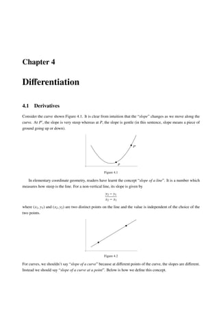
  • 1. Chapter 4 Differentiation 4.1 Derivatives Consider the curve shown Figure 4.1. It is clear from intuition that the “slope” changes as we move along the curve. At P , the slope is very steep whereas at P, the slope is gentle (in this sentence, slope means a piece of ground going up or down). P P Figure 4.1 In elementary coordinate geometry, readers have learnt the concept “slope of a line”. It is a number which measures how steep is the line. For a non-vertical line, its slope is given by y2 − y1 x2 − x1 where (x1, y1) and (x2, y2) are two distinct points on the line and the value is independent of the choice of the two points. Figure 4.2 For curves, we shouldn’t say “slope of a curve” because at different points of the curve, the slopes are different. Instead we should say “slope of a curve at a point”. Below is how we define this concept.
  • 2. 104 Chapter 4. Differentiation First we have a curve 𝒞 and a point P on the curve. To define the slope of 𝒞 at P, take a point Q on the curve different from P. The line PQ is called a secant line at P. Its slope, denoted by mPQ, can be found using the coordinates of P and Q. If we let Q move along the curve, the slope mPQ changes. 𝒞 Q P Figure 4.3 Suppose that as Q approaches P, the number mPQ approaches a fixed value. This value, denoted by m𝒞,P or simply mP if the curve is understood, is called the slope of 𝒞 at P; and the line with slope mP and passing through P is called the tangent line to the curve 𝒞 at P. Remark The number m𝒞,P (if exist) is the unique real number satisfying (∗) mPQ is arbitrarily close to m𝒞,P if Q belonging to 𝒞 is sufficiently close to (but different from) P. In view of the concept “limit of a function at a point” and the notation lim x→a f(x), we may write lim Q→P along 𝒞 mPQ = m𝒞,P to mean that (∗) holds. Below, we will discuss how to find lim Q→P along 𝒞 mPQ by rewriting it as the limit of a difference quotient. Formula for Slope Suppose 𝒞 is given by y = f(x), where f is a function; and P(x0, f(x0)) is a point on 𝒞. For any point Q on 𝒞 with Q P, its x-coordinate can be written as x0 + h where h 0 (if h > 0, Q is on the right of P; if h < 0, Q is on the left of P). Thus, Q can be written as (x0 + h, f(x0 + h)). The slope mPQ of the secant line PQ is mPQ = f(x0 + h) − f(x0) (x0 + h) − x0 = f(x0 + h) − f(x0) h Note that as Q approaches P, the number h approaches 0. From these, we see that the slope of 𝒞 at P (denoted by mP) is mP = lim h→0 f(x0 + h) − f(x0) h (4.1.1) provided that the limit exists. Remark The limit in (4.1.1) is a two-sided limit. This is because Q can approach P from the left or from the right and so h can approach 0 from the left or from the right.
  • 3. 4.1. Derivatives 105 Example Find the slope of the curve given by y = x2 at the point P(3, 9). Solution Put f(x) = x2. By (4.1.1), the required slope (denoted by mP) is mP = lim h→0 f(3 + h) − f(3) h = lim h→0 (3 + h)2 − 32 h = lim h→0 (9 + 6h + h2) − 9 h = lim h→0 6h + h2 h = lim h→0 (6 + h) = 6. -3-2-1 1 2 3 2 4 6 8 10 12 14 Figure 4.4 Definition Let x0 be a real number and let f be a function defined on an open interval containing x0. Suppose the limit in (4.1.1) exists. Then we say that f is differentiable at x0. Convention Open intervals will be denoted by (a, b) including the cases where a = −∞ and/or b = ∞, unless otherwise stated. Thus (a, b) can be any one of the following: • (a, b) where a, b ∈ R and a < b; • (−∞, b) where a = −∞ and b ∈ R; • (a, ∞) where a ∈ R and b = ∞; • (−∞, ∞) where a = −∞ and b = ∞. Remark • The condition “f is a function defined on an open interval containing x0” means that there is an open interval (a, b) such that (a, b) ⊆ dom (f) and x0 ∈ (a, b). Hence, f is defined on the left-side and right-side of x0 as well as at x0. The expression f(x0 + h) − f(x0) h in the limit in (4.1.1), considered as a function of h, is defined on the left-side and the right-side of 0 but is undefined at 0. • “f is differentiable at x0” means that the slope of the curve 𝒞 at P exists, where 𝒞 is given by y = f(x) and P is the point on 𝒞 whose x-coordinate is x0. • There is an alternative way to describe the limit in (4.1.1). Putting x = x0 + h, we have x − x0 = h. Note that as h approaches to 0, x approaches to x0. Hence we have lim h→0 f(x0 + h) − f(x0) h = lim x→x0 f(x) − f(x0) x − x0 . Theorem 4.1.1 Let x0 be a real number and let f be a function defined on an open interval containing x0. Suppose f is differentiable at x0. Then f is continuous at x0.
  • 4. 106 Chapter 4. Differentiation Proof Since f is differentiable at x0, by definition, lim x→x0 f(x) − f(x0) x − x0 exists (a real number). Hence we have lim x→x0 f(x) − f(x0) = lim x→x0 f(x) − f(x0) x − x0 · (x − x0) = lim x→x0 f(x) − f(x0) x − x0 · lim x→x0 (x − x0) Limit Rule (La5) = lim x→x0 f(x) − f(x0) x − x0 · (x0 − x0) Theorem 3.5.1 = lim x→x0 f(x) − f(x0) x − x0 · 0 = 0. Therefore, we get lim x→x0 f(x) = lim x→x0 f(x) − f(x0) + f(x0) = lim x→x0 f(x) − f(x0) + lim x→x0 f(x0) Limit Rule (La4) = 0 + f(x0) From above and Limit Rule (La1) = f(x0). That is, f is continuous at x0. The following example illustrates that converse of Theorem 4.1.1 is not true. Example Let f(x) = |x|. The domain of f is R. The function f is continuous at 0. This is because • lim x→0− f(x) = lim x→0− (−x) = 0; • lim x→0+ f(x) = lim x→0+ x = 0, and so lim x→0 f(x) = 0 = f(0). -2 -1 1 2 1 2 Figure 4.5 However, f is not differentiable at 0. This is because lim h→0 f(0 + h) − f(0) h does not exist as the left-side and right-side limits are unequal: lim h→0+ f(0 + h) − f(0) h = lim h→0+ h − 0 h = lim h→0+ 1 = 1 and lim h→0− f(0 + h) − f(0) h = lim h→0− −h − 0 h = lim h→0− −1 = −1. Definition Let f be a function. (1) Suppose that f is differentiable at every point belonging to an open interval (a, b). Then we say that f is differentiable on (a, b).
  • 5. 4.1. Derivatives 107 (2) Suppose that f is differentiable at every point belonging to its domain. Then we say that f is a differen- tiable function. Remark If f is a differentiable function, then its domain can be written as a union of open intervals. Example Let f(x) = |x|. In a previous example, we have seen that f is not differentiable at 0. Thus f is not a differentiable function. Below we will show that f is differentiable at every x0 0. Thus, f is differentiable on (0, ∞) as well as on (−∞, 0). (x0 > 0) In this case, if h is a small enough real number, then x0 + h > 0 and so we have f(x0 + h) − f(x0) = |x0 + h| − |x0| = (x0 + h) − x0 = h, which yields lim h→0 f(x0 + h) − f(x0) h = lim h→0 h h = lim h→0 1 = 1. (x0 < 0) In this case, if h is a small enough real number, then x0 + h < 0 and so we have f(x0 + h) − f(x0) = |x0 + h| − |x0| = −(x0 + h) − (−x0) = −h, which yields lim h→0 f(x0 + h) − f(x0) h = lim h→0 −h h = lim h→0 −1 = −1. A function f is differentiable means that for every x ∈ dom (f), the limit of the difference quotient lim h→0 f(x + h) − f(x) h exists; the limit is a real number and its value depends on x. In this way, we get a func- tion, called the derivative of f and denoted by f , from dom (f) to R. The graph of f is a curve. The assumption that f is a differentiable function implies that at every point on the curve, the slope exists; at the point whose x-coordinate is x0, the slope is f (x0). Thus f can be considered as slope function. y = f(x) (x0, f(x0)) slope = f (x0) (x1, f(x1)) slope = f (x1) Figure 4.6 More generally, if f is differentiable only at some points in its domain, we can still define the derivative of f on a smaller set. Definition Let f be a function that is differentiable at some points belonging in its domain. Then the derivative of f, denoted by f , is the function (from a subset of dom (f) into R) given by f (x) = lim h→0 f(x + h) − f(x) h ,
  • 6. 108 Chapter 4. Differentiation where the domain of f is x ∈ dom ( f) : lim h→0 f(x + h) − f(x) h exists . Example Let f(x) = |x|. Using results in a previous example, we see that f (x) =    1 if x > 0, −1 if x < 0, where dom (f ) = {x ∈ R : x 0}. Example Let f(x) = x2. Find the derivative of f. Explanation To find the derivative of f means to find the domain of f and find a formula for f (x). Solution By definition, we have f (x) = lim h→0 f(x + h) − f(x) h = lim h→0 (x + h)2 − x2 h = lim h→0 (x2 + 2xh + h2) − x2 h = lim h→0 2xh + h2 h = lim h→0 (2x + h) = 2x. The domain of f is R. Remark The logic in the above solution is as follows: (1) First we find that lim h→0 f(x + h) − f(x) h = 2x for all x ∈ R. (2) From (1), we see that the domain of f is R and f (x) = 2x for all x ∈ R. Example Let f(x) = x3. Find f (x). Solution By definition, we have f (x) = lim h→0 f(x + h) − f(x) h = lim h→0 (x + h)3 − x3 h = lim h→0 (x3 + 3x2h + 3xh2 + h3) − x3 h = lim h→0 3x2h + 3xh2 + h3 h = lim h→0 (3x2 + 3xh + h2) = 3x2.
  • 7. 4.1. Derivatives 109 Remark The domain of f is R. Terminology The process of finding derivatives is called differentiation. In a previous example to find the slope of the parabola y = f(x) = x2 at the point (3, 9), we use definition to find f (3). In fact, if we know that f (x) = 2x, then by direct substitution, we get f (3) = 6. In the next section, we will discuss how to find f (x) using rules for differentiation. Terminology f (x0) is called the derivative of f at x0. To represent a function f, we sometimes write y or f(x). Similarly, the derivative of a function can be represented in many ways. Notation • To denote the derivative of a function f, we have the following notations. f , y , dy dx , Df, Dy, f (x) and d dx f(x). • To denote the derivative of f at x0, we have the following notations. f (x0), y (x0), dy dx x=x0 , Df(x0) and Dy(x0). Some readers may wonder why we have the notation as well as the d dx notation. Calculus was “invented” by Newton and Leibniz independently in the late 17th century. Newton used ˙x whereas Leibniz used dx dt to denote the derivative of x with respect to t (time). The notation y is simple whereas dy dx reminds us that it is defined as a limit of difference quotient: dy dx = lim ∆x→0 ∆y ∆x where ∆x = h = (x + h) − x and ∆y = f(x + h) − f(x) are changes in x and y respectively. ∆y ∆x Figure 4.7 Caution dy dx is not a fraction. • dy dx is f or f (x); it is a function or an expression in x. It can be written as d dx y also. The notation d dx can be considered as an operation; to find dy dx means to perform the differentiation operation on y. Some authors use the notation Dy instead, where D stands for the differentiation operator (some authors use Dxy to emphasize that the variable is x). • Although we can define dy and dx (called differentials), dy dx does not mean “divide dy by dx”. In Chap- ter 10, we will describe differentials briefly (the purpose is to introduce the substitution method for integration).
  • 8. 110 Chapter 4. Differentiation Using d dx notation, the results obtained in the last two examples can be written as d dx x2 = 2x d dx x3 = 3x2. In Exercise 3.5, Question 2(c) and (d), in terms of the d dx notation, the answers can be written as d dx x−1 = −x−2 d dx x 1 2 = 1 2 x−1 2 . These are particular cases of a general result, called the power rule which will be discussed in Section 4.2. Rate of Change • The slope of a line is the rate of change of y with respect to x. The slope of a curve y = f(x) at a point P x0, f(x0) is the limit of the slopes of the secant lines through P, so it is the rate of change of y with respect to x at P. That is, f (x0) or dy dx x=x0 is the rate of change of y with respect to x when x = x0. • If x = t is time and y = s(t) is the displacement function of a moving object then s (t0) or ds dt t=t0 is the rate of change of displacement with respect to time when t = t0, that is, the (instantaneous) velocity at t = t0. In the Introduction of Chapter 3, we consider the velocity of an object at time t = 2, where the displacement function is s(t) = t2. Using differentiation, the velocity at t = 2 can be found easily: s (2) = d dt t2 t=2 = 2t t=2 = 4. Remark The notation 2t t=2 means substitute t = 2 into the expression 2t. More generally, the notation f(x) x=x0 means f(x0). Exercise 4.1 1. For each of the following f, use definition to find f (x). (a) f(x) = 2x2 + 1 (b) f(x) = x3 − 3x (c) f(x) = x4 (d) f(x) = 1 x2 4.2 Rules for Differentiation Derivative of Constant The derivative of a constant function is 0 (the zero function), that is d dx c = 0, where c is a constant.
  • 9. 4.2. Rules for Differentiation 111 Explanation In the above formula, we use c to denote the constant function f given by f(x) = c. The domain of f is R. The result means that f is differentiable on R and that f (x) = 0 for all x ∈ R. Proof Let f : R −→ R be the function given by f(x) = c for x ∈ R. By definition, we get f (x) = lim h→0 f(x + h) − f(x) h = lim h→0 c − c h = lim h→0 0 h = lim h→0 0 = 0 Geometric meaning The graph of the constant function c is the horizontal line given by y = c. At every point on the line, the slope is 0. Derivative of Identity Function The derivative of the identity function is the constant function 1, that is d dx x = 1. Explanation In the above formula, we use x to denote the identity function, that is, the function f given by f(x) = x. The domain of f is R. The result means that f is differentiable on R and f (x) = 1 for all x ∈ R. Proof Let f : R −→ R be the function given by f(x) = x for x ∈ R. By definition, we get f (x) = lim h→0 f(x + h) − f(x) h = lim h→0 x + h − x h = lim h→0 h h = lim h→0 1 = 1 Geometric meaning The graph of the identity function is the line given by y = x. At every point on the line, the slope is 1. Power Rule for Differentiation (positive integer version) Let n be a positive integer. Then the power function xn is differentiable on R and we have d dx xn = nxn−1 . Explanation In the above formula, we use xn to denote the n-th power function, that is, the function f given by f(x) = xn. The domain of f is R. The result means that f is differentiable on R and f (x) = nxn−1 for all
  • 10. 112 Chapter 4. Differentiation x ∈ R. When n = 1, the formula becomes d dx x = 1x0. In the expression on the right side, x0 is understood to be the constant function 1 and so the formula reduces to d dx x = 1 which is the rule for derivative of the identity function. To prove that the result is true for all positive integers n, we can use mathematical induction. For base step, we know that the result is true when n = 1. For the induction step, we can apply product rule (will be discussed later). Below we will give alternative proofs for the power rule (positive integer version). Proof Let f : R −→ R be the function given by f(x) = xn for x ∈ R. By definition, we get f (x) = lim h→0 f(x + h) − f(x) h = lim h→0 (x + h)n − xn h . To find the limit, we “simplify” the numerator to obtain a factor h and then cancel it with the factor h in the denominator. For this, we can use: • a factorization formula an − bn = (a − b)(an−1 + an−2b + · · · + abn−2 + bn−1) • the Binomial Theorem (a + b)n = an + n 1 an−1b + n 2 an−2b2 + · · · + n n−2 a2bn−2 + n n−1 abn−1 + bn where n 1 = n and n 2 = n(n − 1) 2 and n 3 = n(n − 1)(n − 2) 3 · 2 etc. are the binomial coefficients (see Binomial Theorem in the appendix). However, in the proof below, we only need to know the coefficient n 1 = n; the other coefficients are not important. (Method 1) By the factorization formula, we get (x + h)n − xn = (x + h − x) (x + h)n−1 + (x + h)n−2x + · · · + (x + h)xn−2 + xn−1 = h (x + h)n−1 + (x + h)n−2x + · · · + (x + h)xn−2 + xn−1 Therefore, f (x) = lim h→0 (x + h)n−1 + (x + h)n−2x + · · · + (x + h)xn−2 + xn−1 = (x + 0)n−1 + (x + 0)n−2 · x + · · · + (x + 0) · xn−2 + xn−1 Theorem 3.5.1 = xn−1 + xn−1 + · · · + xn−1 + xn−1 n terms = nxn−1 (Method 2) From the Binomial Theorem, we get (x + h)n − xn = xn + n 1 xn−1h + n 2 xn−2h2 + · · · + n n−2 x2hn−2 + n n−1 xhn−1 + hn − xn = n 1 xn−1h + n 2 xn−2h2 + · · · + n n−2 x2hn−2 + n n−1 xhn−1 + hn = h nxn−1 + n 2 xn−2h + · · · + n n−2 x2hn−3 + n n−1 xhn−2 + hn−1 because n 1 = n Therefore, f (x) = lim h→0 nxn−1 + n 2 xn−2h + · · · + n n−2 x2hn−3 + n n−1 xhn−2 + hn−1 = nxn−1 + n 2 xn−2 · 0 + · · · + n n−2 x2 · 0 + n n−1 x · 0 + 0 Theorem 3.5.1 = nxn−1.
  • 11. 4.2. Rules for Differentiation 113 Example Let y = x123. Find dy dx . Explanation The notation y = x123 represents a power function. To find dy dx means to find the derivative of the function. Solution dy dx = d dx x123 = 123x123−1 Power Rule = 123x122 Caution In the above solution, the first step is “substitution”. It can also be written as dx123 dx . It is wrong to write dy dx x123 which means dy dx multiplied by x123. The notation d dx x123 is the derivative of the power function x123. If we consider d dx as an operator, d dx x123 means “perform the differentiation operation on the function x123”. Remark • In the power rule, if we put n = 0, the left side is d dx x0 and right side is 0x−1. The function x0 is understood to be the constant function 1. Thus d dx x0 = 0 by the rule for derivative of constant. The domain of the function x−1 is R {0}. Therefore, 0x−1 is the function whose domain is R {0} and is always equal to 0. If we extend the domain to R and treat 0x−1 as the constant function 0, then the power rule is true when n = 0. • Later in this section, we will show that the power rule is also true for negative integers n using the quotient rule (in fact, it is true for all real numbers n; the result will be called the general power rule). • In Chapter 6, we will discuss integration which is the reverse process of differentiation. There is a result called the power rule for integration. However, in this chapter, “power rule” always means “power rule for differentiation”. Constant Multiple Rule for Differentiation Let f be a function and let k be a constant. Suppose that f is differentiable. Then the function k f is also differentiable. Moreover, we have d dx (k f)(x) = k · d dx f(x). Explanation The function k f is defined by (k f)(x) = k · f(x) for x ∈ dom (f). The result means that if f (x) exists for all x ∈ dom ( f), then (k f) (x) = k · f (x) for all x ∈ dom ( f), that is, (k f) = k · f . Proof By definition, we have (k f) (x) = lim h→0 (k f)(x + h) − (k f)(x) h = lim h→0 k · f(x + h) − k · f(x) h Definition of k f = lim h→0 k · f(x + h) − f(x) h = k · lim h→0 f(x + h) − f(x) h Limit Rule (La5s) = k · f (x)
  • 12. 114 Chapter 4. Differentiation Remark There is a pointwise version of the constant multiple rule: the result remains valid if differentiable function is replaced by differentiable at a point. Let f be a function and let k be a constant. Suppose that f is differentiable at x0. Then the function k f is also differentiable at x0. Moreover, we have (k f) (x0) = k · f (x0) There are also pointwise versions for the sum rule, product rule and quotient rule which will be discussed later. Readers can formulate the results themselves. Example Let y = 3x4. Find dy dx . Solution dy dx = d dx 3x4 = 3 · d dx x4 Constant Multiple Rule = 3 · (4x4−1) Power Rule = 12x3 Sum Rule for Differentiation (Term by Term Differentiation) Let f and g be functions with the same domain. Suppose that f and g are differentiable. Then the function f + g is also differentiable. Moreover, we have d dx ( f + g)(x) = d dx f(x) + d dx g(x). Explanation The function f + g is defined by (f + g)(x) = f(x) + g(x) for x belonging to the common domain A of f and g. The result means that if f (x) and g (x) exist for all x ∈ A, then (f + g) (x) = f (x) + g (x) for all x ∈ A, that is, (f + g) = f + g . Proof By definition, we have ( f + g) (x) = lim h→0 ( f + g)(x + h) − ( f + g)(x) h = lim h→0 f(x + h) + g(x + h) − f(x) + g(x) h Definition of f + g = lim h→0 f(x + h) − f(x) + g(x + h) − g(x) h = lim h→0 f(x + h) − f(x) h + g(x + h) − g(x) h = lim h→0 f(x + h) − f(x) h + lim h→0 g(x + h) − g(x) h Limit Rule (La4) = f (x) + g (x) Remark • If the domains of f and g are not the same but their intersection is nonempty, we define f + g to be the function with domain dom (f) ∩ dom (g) given by (f + g)(x) = f(x) + g(x). The following is a more general version of the sum rule:
  • 13. 4.2. Rules for Differentiation 115 Let f and g be functions. Suppose that f and g are differentiable on an open interval (a, b). Then the function f + g is also differentiable on (a, b). Moreover, on the interval (a, b), we have d dx (f + g)(x) = d dx f(x) + d dx g(x). There are also more general versions for the product rule and quotient rule. Readers can formulate the results themselves. • The result is also true for difference of two functions, that is, d dx (f − g)(x) = d dx f(x) − d dx g(x). The result for difference can be proved similar to that for sum. Alternatively, it can be proved from the sum rule together with the constant multiple rule: ( f − g) (x) = ( f + (−1)g) (x) = f (x) + (−1)g (x) Sum Rule = f (x) + (−1) · g (x) Constant Multiple Rule = f (x) − g (x). • Term by Term Differentiation can be applied to sum and difference of finitely many terms. Example Let y = x2 + 3. Find dy dx . Solution dy dx = d dx (x2 + 3) = d dx x2 + d dx 3 Term by Term Differentiation = 2x + 0 Power Rule and Derivative of Constant = 2x Example Let f(x) = x5 − 6x7. Find f (x). Explanation This question is similar to the last one. If we put y = f(x), then f (x) = dy dx . Below, we use the notation d dx to perform differentiation. Solution f (x) = d dx (x5 − 6x7) = d dx x5 − d dx 6x7 Term by Term Differentiation = 5x4 − 6 · d dx x7 Power Rule and Constant Multiple Rule = 5x4 − 6 · (7x6) Power Rule = 5x4 − 42x6
  • 14. 116 Chapter 4. Differentiation The last two examples illustrate that polynomials can be differentiated term by term. Derivative of Polynomial Let y = anxn + an−1xn−1 + · · · + a2x2 + a1x + a0 be a polynomial. Then we have dy dx = nanxn−1 + (n − 1)an−1xn−2 + · · · + 2a2x + a1. Proof dy dx = d dx anxn + an−1xn−1 + · · · + a2x2 + a1x + a0 = d dx anxn + d dx an−1xn−1 + · · · + d dx a2x2 + d dx a1x + d dx a0 Term by Term Differentiation = an d dx xn + an−1 d dx xn−1 + · · · + a2 d dx x2 + a1 d dx x + 0 Constant Multiple Rule and Derivative of Constant = annxn−1 + an−1(n − 1)xn−2 + · · · + a2 · (2x) + a1 · 1 Power Rule Example Let f(x) = 2x (x2 − 5x + 7). Find the derivative of f at 2. Explanation The question is to find f (2). We can find f (x) using one of the following two ways: • product rule (will be discussed later); • expand the expression to get a polynomial. Then putting x = 2, we get the answer. Below we use the second method to find f (x). Solution f (x) = d dx 2x (x2 − 5x + 7) = d dx 2x3 − 10x2 + 14x = 2 · (3x2) − 10 · (2x) + 14 · 1 Derivative of Polynomial = 6x2 − 20x + 14 The derivative of f at 2 is f (2) = 6(22) − 20(2) + 14 = −2 Product Rule Let f and g be functions with the same domain. Suppose that f and g are differentiable. Then the function fg is also differentiable. Moreover, we have d dx (fg)(x) = g(x) · d dx f(x) + f(x) · d dx g(x). Explanation The function fg is defined by (fg)(x) = f(x) · g(x) for x belonging to the common domain A of f and g. The result means that if f (x) and g (x) exist for all x ∈ A, then (fg) (x) = g(x)f (x) + f(x)g (x) for all x ∈ A, that is, (fg) = gf + fg . Proof By definition, we have (fg) (x) = lim h→0 (fg)(x + h) − (fg)(x) h = lim h→0 f(x + h)g(x + h) − f(x)g(x) h Definition of fg
  • 15. 4.2. Rules for Differentiation 117 To find the limit, we use the following technique: “subtract and add” f(x + h)g(x) in the numerator. ( fg) (x) = lim h→0 f(x + h)g(x + h) − f(x + h)g(x) + f(x + h)g(x) − f(x)g(x) h = lim h→0 f(x + h)g(x + h) − f(x + h)g(x) h + f(x + h)g(x) − f(x)g(x) h = lim h→0 f(x + h) · g(x + h) − g(x) h + lim h→0 g(x) · f(x + h) − f(x) h Limit Rule (La4) = lim h→0 f(x + h) · lim h→0 g(x + h) − g(x) h + lim h→0 g(x) · lim h→0 f(x + h) − f(x) h Limit Rule (La5) = f(x)g (x) + g(x) f (x) Theorem 4.1.1 & Limit Rule (La1) In the last step, the first limit is found by substitution because f is continuous; the third limit is g(x) because considered as a function of h, g(x) is a constant. Example Let y = (x + 1)(x2 + 3). Find dy dx . Explanation The expression defining y is a product of two functions. So we can apply the product rule. Alter- natively, we can expand the expression to get a polynomial and then differentiate term by term. Solution 1 dy dx = d dx (x + 1)(x2 + 3) = (x2 + 3) · d dx (x + 1) + (x + 1) · d dx (x2 + 3) Product Rule = (x2 + 3) · (1 + 0) + (x + 1) · (2x + 0) Derivative of Polynomial = 3x2 + 2x + 3 Solution 2 dy dx = d dx (x + 1)(x2 + 3) = d dx (x3 + x2 + 3x + 3) = 3x2 + 2x + 3 Derivative of Polynomial Quotient Rule Let f and g be functions with the same domain. Suppose that f and g are differentiable and that g has no zero in its domain. Then the function f g is also differentiable. Moreover, we have, d dx f g (x) = g(x) · d dx f(x) − f(x) · d dx g(x) g(x) 2 . Explanation The condition “g has no zero in its domain” means that g(x) 0 for all x ∈ dom (g). The function f g is defined by f g (x) = f(x) g(x) for x ∈ A, where A is the common domain of f and g. The result means that if f (x) and g (x) exist for all x ∈ A, then f g (x) = g(x) f (x) − f(x)g (x) g(x)2 for all x ∈ A, that is, f g = g f − fg g2 .
  • 16. 118 Chapter 4. Differentiation Proof The proof is similar to that for the product rule. Example Let y = x2 + 3x − 4 2x + 1 . Find dy dx . Solution dy dx = d dx x2 + 3x − 4 2x + 1 = (2x + 1) · d dx (x2 + 3x − 4) − (x2 + 3x − 4) · d dx (2x + 1) (2x + 1)2 Quotient Rule = (2x + 1)(2x + 3) − (x2 + 3x − 4)(2) (2x + 1)2 Derivative of Polynomial = (4x2 + 8x + 3) − (2x2 + 6x − 8) (2x + 1)2 = 2x2 + 2x + 11 (2x + 1)2 Power Rule for Differentiation (negative integer version) Let n be a negative integer. Then the power func- tion xn is differentiable on R {0} and we have d dx xn = nxn−1 . Explanation Since n is a negative integer, it can be written as −m where m is a positive integer. The function xn = x−m = 1 xm is defined for all x 0, that is, the domain of xn is R {0}. Proof Let f : R {0} −→ R be the function given by f(x) = x−m, where m = −n. By definition, we have f (x) = d dx 1 xm = xm · d dx 1 − 1 · d dx xm (xm)2 Quotient Rule = xm · 0 − 1 · mxm−1 x2m Derivative of Constant & Power Rule (positive integer version) = −mx(m−1)−2m = −mx−m−1 = nxn−1 Example Find an equation for the tangent line to the curve y = 3x2 − 1 x at the point (1, 2). Explanation The curve is given by y = f(x) where f(x) = 3x2 − 1 x . Since f(1) = 2, the point (1, 2) lies on the curve. To find an equation for the tangent line, we have to find the slope at the point (and then use point-slope form). The slope at the point (1, 2) is f (1). We can use rules for differentiation to find f (x) and then substitute x = 1 to get f (1). Solution To find dy dx , we can use quotient rule or term by term differentiation.
  • 17. 4.2. Rules for Differentiation 119 (Method 1) dy dx = d dx 3x2 − 1 x = x · d dx (3x2 − 1) − (3x2 − 1) · d dx x x2 Quotient Rule = x · 3 · (2x) − (3x2 − 1) · 1 x2 Derivative of Polynomial = 3x2 + 1 x2 (Method 2) dy dx = d dx (3x2 − 1)x−1 = d dx (3x − x−1) = d dx 3x − d dx x−1 Term by Term Differentiation = 3 − (−1)x−2 Derivative of Polynomial & Power Rule = 3 + 1 x2 . The slope of the tangent line at the point (1, 2) is dy dx x=1 = 3 + 1 1 = 4. Equation for the tangent line: y − 2 = 4(x − 1) (point-slope form) 4x − y − 2 = 0 (general linear form) The next result is a special case of the general power rule. Since the square root function appears often in applied problems and the proof is not difficult, we give the result here. Derivative of the Square Root Function The derivative of the square root function √ x is 1 2 √ x , that is, d dx √ x = 1 2 √ x . Explanation The domain of the square root function is [0, ∞). Since the function is undefined on the left-side of 0, we can only consider differentiability of the function on (0, ∞). The result means that f (x) = 1 2 √ x for all x ∈ (0, ∞) where f(x) = √ x. Proof Let f : [0, ∞) −→ R be the function given by f(x) = √ x. For every x > 0, note that if h is a small enough real number, then x + h ∈ dom (f) and hence if h is a small enough non-zero real number, we have f(x + h) − f(x) h = √ x + h − √ x h = √ x + h − √ x √ x + h + √ x h √ x + h + √ x = (x + h) − x h √ x + h + √ x = h h √ x + h + √ x = 1 √ x + h + √ x
  • 18. 120 Chapter 4. Differentiation which, by definition, implies that f (x) = lim h→0 1 √ x + h + √ x = 1 lim h→0 √ x + h + √ x Limit Rule (La6) = 1 lim h→0 √ x + h + lim h→0 √ x Limit Rule (La4) = 1 √ x + 0 + √ x By continuity & Limit Rule (La1) = 1 2 √ x In the second last step, the first limit is found by substitution because the square root function is continuous; the second limit is the limit of a constant. Example Let y = √ x (x + 1). Find dy dx . Solution dy dx = d dx √ x (x + 1) = (x + 1) · d dx √ x + √ x · d dx (x + 1) Product Rule = (x + 1) · 1 2 √ x + √ x · 1 Derivative of Square Root Function & Derivative of Polynomial = √ x 2 + 1 2 √ x + √ x = 3 √ x 2 + 1 2 √ x Remark If we expand the expression defining y, we get x 3 2 + x 1 2 . The derivative can be found if we know the derivative of x 3 2 . Power Rule for Differentiation (n + 1 2 version) Let n be an integer. Then the function xn+ 1 2 is differentiable on (0, ∞) and we have d dx xn+ 1 2 = n + 1 2 xn− 1 2 . Explanation Denoting the function by f, if n = 0, then f is the square root function; if n is positive, then the domain of f is [0, ∞); if n is negative, then the domain of f is (0, ∞). Putting r = n + 1 2 , then we have f(x) = xr and the result means that f (x) = rxr−1 for all x > 0. This result has the same form as the power rule and it will be referred to as the power rule. Remark There is a more general result called the General Power Rule (see Chapter 9). Proof Let f be the function given by f(x) = xn+1 2 . Note that f(x) = xn · √ x and so by the Product Rule and the
  • 19. 4.2. Rules for Differentiation 121 Rule for Derivative of the Square Root Function, the function f is differentiable on (0, ∞) and we have f (x) = d dx xn · √ x = √ x · d dx xn + xn · d dx √ x Product Rule = √ x · nxn−1 + xn · 1 2 √ x Power Rule & Derivative Square Root Function = nxn−1 2 + 1 2 xn−1 2 = n + 1 2 xn− 1 2 Below, we redo the preceding example using the n + 1 2 version of the power rule. Example Let y = √ x (x + 1). Find dy dx . Solution dy dx = d dx x 1 2 (x + 1) = d dx x 3 2 + x 1 2 = d dx x 3 2 + d dx x 1 2 Term by Term Differentiation = 3 2 x 3 2 −1 + 1 2 x 1 2 −1 Power Rule = 3 2 x 1 2 + 1 2 x−1 2 Example Let y = 2x2 − 3 √ x . Find dy dx . Solution 1 dy dx = d dx 2x2 − 3 √ x = √ x · d dx (2x2 − 3) − (2x2 − 3) · d dx √ x ( √ x)2 Quotient Rule = √ x · 2 · (2x) − (2x2 − 3) · 1 2 √ x x Derivative of Polynomial & Derivative of Square Root Function = 4x √ x − x √ x + 3 2 √ x x = 3 √ x + 3 2x √ x
  • 20. 122 Chapter 4. Differentiation Solution 2 dy dx = d dx (2x2 − 3)x− 1 2 = d dx 2x 3 2 − 3x− 1 2 = 2 · d dx x 3 2 − 3 · d dx x− 1 2 Term by Term Differentiation = 2 · 3 2 x 1 2 − 3 · − 1 2 x−3 2 Power Rule = 3x 1 2 + 3 2 x−3 2 We close this section with the following “Caution” and “Question”. The “caution” points out a common mistake that many students made. Caution d dx 2x x · 2x−1, we can’t apply the Power Rule because 2x is not a power function; it is an exponential function (see Chapter 8). Question Using rules discussed in this chapter, we can differentiate polynomial functions as well as rational functions. For example, to differentiate f(x) = (x2 + 5)3, we can first expand the cube to get a polynomial of degree 6 and then differentiate term by term. How about the following (1) f(x) = (x2 + 5)30 ? (2) f(x) = √ x2 + 5 ? For (1), we can expand and then differentiate term by term (if we have enough patience). However, this doesn’t work for (2). Note that both functions are in the form x → (x2 + 5)r which can be considered as composition of two functions: x → (x2 + 5) → (x2 + 5)r . In Chapter 9, we will discuss the chain rule, a tool to handle this kind of differentiation. Exercise 4.2 1. For each of the following y, find dy dx . (a) y = −π (b) y = 2x9 + 3x (c) y = x2 + 5x − 7 (d) y = x (x − 1) (e) y = (2x − 3)(5 − 6x) (f) y = (x2 + 5)3 (g) y = 23 x4 (h) y = x − 1 x (i) y = x − 1 x + 1 (j) y = √ x √ x + 1 2. For each of the following f, find f (a) for the given a. (a) f(x) = x3 − 4x, a = 1 (b) f(x) = 2 x3 + 4 x , a = 2 (c) f(x) = 3x 1 3 − 5x 2 3 , a = 27 (d) f(x) = πx2 − 2 √ x, a = 4 (e) f(x) = (x2 + 3)(x3 + 2), a = 1 (f) f(x) = x2 + 1 2x − 3 , a = 2 (g) f(x) = x2 + 3x − 5 x2 − 7x + 5 , a = 1
  • 21. 4.3. Higher-Order Derivatives 123 3. Consider the curve given by y = 3x4 − 6x2 + 2. (a) Find the slope of the curve at the point whose x-coordinate is 2. (b) Find an equation for the tangent line at the point (1, −1). (c) Find the point(s) on the curve at which the tangent line is horizontal. 4. It is known that d dx sin x = cos x. For each of the following y, find dy dx . (a) y = x sin x (b) y = sin x x + 1 (c) y = x2 + 1 sin x (d) y = x (x + 2) sin x 5. Let f be a differentiable function. (a) Use product rule to show that d dx f(x)2 = 2f(x) · d dx f(x). (b) Use product rule and the result in (a) to show that d dx f(x)3 = 3f(x)2 · d dx f(x). (c) Can you guess (and prove) a formula for d dx f(x)n, where n is a positive integer? 6. (a) Use the result in 5(a) to find d dx (x3 + 5x2 − 2)2. (b) Use the result in 5(b) to find d dx (x2 + 5)3. Compare your answer with that in Q.1(f). 4.3 Higher-Order Derivatives Let f be a function that is differentiable at some points belonging to dom (f). Then f is a function. • If, in addition, f is differentiable at some points belonging to dom (f ), then the derivative of f exists and is denoted by f ; it is the function given by f (x) = lim h→0 f (x + h) − f (x) h and is called the second derivative of f. • If, in addition, f is differentiable at some points belonging to dom (f ), then the derivative of f is denoted by f , called the third derivative of f. • In general, the n-th derivative of f (where n is a positive integer), denoted by f(n), is defined to be the derivative of the (n−1)-th derivative of f (where the 0-th derivative of f means f). For n = 1, the first derivative of f is simply the derivative f of f. For n > 1, f(n) is called a higher-order derivative of f. Notation Similar to first order derivative, we have different notations for second order derivative of f. y , f , d2y dx2 , D2 f, D2 y, f (x) and d2 dx2 f(x). Readers may compare these with that on page 109. Similarly, we also have different notations for other higher- order derivatives. Example Let f(x) = 5x3 − 2x2 + 6x + 1. Find the derivative and all the higher-order derivatives of f. Explanation The question is to find for each positive integer n, the domain of the n-th derivative of f and a formula for f(n)(x). To find f (x), we can apply differentiation term by term. To find f (x), by definition, we have f (x) = d dx f (x) which can be simplified using the result for f (x) and rules for differentiation.
  • 22. 124 Chapter 4. Differentiation Solution f (x) = d dx (5x3 − 2x2 + 6x + 1) = 15x2 − 4x + 6 Derivative of Polynomial f (x) = d dx (15x2 − 4x + 6) = 30x − 4 Derivative of Polynomial f (x) = d dx (30x − 4) = 30 Derivative of Polynomial f(4)(x) = 0 Derivative of Constant From this we see that for n ≥ 4, f(n)(x) = 0. Moreover, for every positive integer n, the domain of f(n) is R. Example Let f(x) = x3 − 1 x . Find f (3) and f (−4). Explanation • To find f (3), we find f (x) first and then substitute x = 3. Although f(x) is written as a quotient of two functions, it is better to find f (x) by expanding (x3 − 1)x−1. • To find f (−4), we find f (x) first and then substitute x = −4. To find f (x), we differentiate the result obtained for f (x). Solution f (x) = d dx (x3 − 1)x−1 = d dx x2 − x−1 = 2x − (−1)x−2 Term by Term Differentiation & Power Rule = 2x + x−2 f (3) = 2 · (3) + 3−2 = 55 9 f (x) = d dx 2x + x−2 By result for f (x) = 2 + (−2)x−3 Term by Term Differentiation & Power Rule = 2 − 2x−3 f (−4) = 2 − 2 · (−4)−3 = 65 32 Meaning of Second Derivative • The graph of y = f(x) is a curve. Note that f (x) = dy dx is the slope function; it is the rate of change of y with respect to x. Since f (x) = d2 y dx2 is the derivative of the slope function, it is the rate of change
  • 23. 4.3. Higher-Order Derivatives 125 of slope and is related to a concept called convexity (bending) of a curve. More details can be found in Chapter 5. • If x = t is time and if y = s(t) is the displacement function of a moving object, then s (t) = ds dt is the velocity function. The derivative of velocity is s (t) or d2 s dt2 ; it is the rate of change of the velocity (function), that is, the acceleration (function). Exercise 4.3 1. For each of the following y, find d2 y dx2 . (a) y = x3 − 3x2 + 4x − 1 (b) y = (2x + 3)(4 − x) (c) y = √ x (1 + x) (d) y = 1 − 2x x2 (e) y = (x3 + 1)2 2. For each of the following f, find f (a) for the given a. (a) f(x) = 7x6 − 8x5 + 15x, a = 1 (b) f(x) = x2(1 − 2x), a = 2 (c) f(x) = (2 + 3x)2, a = 0 3. Let f(x) = anxn + an−1xn−1 + · · · + a1x + a0 be a polynomial of degree n. (a) Find f(0) and f (0). (b) Find f(n)(x) and f(n+1)(x).