1. Lab No.04
MATLAB graphics
Designed by : Dawar Awan
dawar@cecos.edu.pk
CECOS College of Engineering and IT
March – July 2012

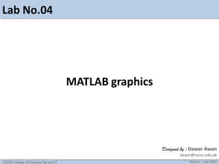
2. Discrete signals
 Plot the discrete signal x = [1 2 3 4] in MATLAB
4
3
2
1
-1
0
1
2
 using stem(x) plots the signal starting from index number 1
CECOS College of Engineering and IT
March – July 2012

3. Practice
 Plot the following discrete time sequences
x[n]=[1 1 1 1 2 1 1 1 1]
x[n]=[5 4 3 2 1 0 1 2 3 4 5]
CECOS College of Engineering and IT
March – July 2012

4. Continuous plot
 >> plot(n,x)
 Shows a continuous plot of x
 Actually the discrete points are only connected with
straight lines.
CECOS College of Engineering and IT
March – July 2012

5. Labeling the plot
 Example:
CECOS College of Engineering and IT
March – July 2012

6. Labeling the plot
CECOS College of Engineering and IT
March – July 2012

7. Multiple plots
 Using single “plot” instruction
 Example:
x = 0:0.01:5;
y1=sin(x);
y2=sin(2*x);
y3=sin(4*x);
plot(x,y1,x,y2,x,y3)
CECOS College of Engineering and IT
March – July 2012

8. Multiple plots
CECOS College of Engineering and IT
March – July 2012

9. Multiple plots
 Using multiple “plot” instructions
 Example:
x = 0:0.01:5;
y1=sin(x);
y2=sin(2*x);
y3=sin(4*x);
plot(x,y1);
hold on;
plot(x,y2);
plot(x,y3);
CECOS College of Engineering and IT
March – July 2012

10. Multiple plots
CECOS College of Engineering and IT
March – July 2012

11. Changing default plot settings
 Example:
x = 0:0.1:5;
y1=sin(x);
y2=sin(2*x);
y3=sin(4*x);
plot(x,y1,’+’,x,y2,':',x,y3,‘--');
CECOS College of Engineering and IT
March – July 2012

12. Changing default plot settings
CECOS College of Engineering and IT
March – July 2012

13. Changing default plot settings
 line types and mark types
Linetypes :
solid (-), dashed (--), dotted (:), dashdot (-.)
Marktypes :
point (.), plus (+), star (*), circle (o), x-mark (x)
Check the help of “plot” for more effects.
CECOS College of Engineering and IT
March – July 2012

14. Axis command
 Used to manually zoom axis
 axis([xmin xmax ymin ymax])
 Example:
CECOS College of Engineering and IT
March – July 2012

15. Axis command
 Without axis command
CECOS College of Engineering and IT
March – July 2012

16. Axis command
 With axis command
CECOS College of Engineering and IT
March – July 2012

17. SUBPLOT
 Example:
x = 0:1:10;
y = x.^2;
z = 10*x;
subplot (1,2,1)
plot(x,y)
subplot (1,2,2)
plot(x,z)
subplot(m,n,p) : makes m rows and n columns of figures in figure window
and p shows the location of the current plot i.e the plot instruction just below
the subplot
CECOS College of Engineering and IT
March – July 2012

18. SUBPLOT
CECOS College of Engineering and IT
March – July 2012

19. Generating a sine wave
 Example: creating a 5Hz sine wave, sampled at 8000Hz.
f=5;
fs=8000;
t=[0:1/fs:1];
y=sin(2*pi*f*t);
plot(t,y);
CECOS College of Engineering and IT
March – July 2012

20. Generating a sine wave
 Observe 5 cycles per second.
CECOS College of Engineering and IT
March – July 2012

21. Generating a sine wave
 Example: Creating a 1000Hz sine wave, sampled at
8000Hz, and routing it to computer’s soundcard.
f=1000;
fs=8000;
t=[0:1/fs:3];
y=sin(2*pi*f*t);
sound(y,fs);
The sound will be heard for 3 seconds, as dictated by the code
CECOS College of Engineering and IT
March – July 2012

22. Task
1. Plot the two curves y1 = x2 and y2 = 2x on the same graph using
different plot styles. Label the plot properly
2. Write a MATLAB program that adds the following two signals,
Plot the original signals as well as their sum.
x1[n] = [2 2 2 2 2]
x2[n] = [2 2 2 2 0 0]
3. Scale the amplitude of the following signal by a factor of 2 and
½ and show the scaled signals along with the original.
x(t) = sin(t) + 1/3sin(3t)
CECOS College of Engineering and IT
,
t=0:0.01:10
March – July 2012

23. Tasks
4. Demonstrate the use of the function ”plot3” to plot a straight
3D line
CECOS College of Engineering and IT
March – July 2012