Normal Distribution.pptx

The Normal
distribution
MBMG-7104/ ITHS-2202/ IMAS-3101/ IMHS-3101
@Ravindra Nath Shukla (PhD Scholar) ABV-IIITM

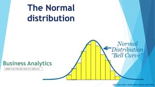
What is normal distribution?
The Normal Distribution, also called
the Gaussian Distribution, is the
most significant continuous
probability distribution.
A normal distribution is a
 symmetric, bell-shaped curve
 that describes the distribution of
continuous random variables.
 The normal curve describes how data
are distributed in a population.

……A normal distribution is a
 A large number of random variables are either nearly or
exactly represented by the normal distribution
 The normal distribution can be used to represent a wide
range of data, such as test scores, height measurements,
and weights of people in a population.

The normal distribution has two parameters,
 mean (μ ) and standard deviation (σ) .
 It is important to know these two parameters because they
are used to calculate probabilities associated with the
normal distribution.
 Mean : - It is the measure of central tendency, i.e. it provides
us an idea of the concentration of the observations about
the central part of the distribution.
 Standard deviation :- Standard deviation describes the
dispersion or spread the variables about the central value.

Normal distribution is defined by its
mean and standard dev.
E(X)= =
Var(X)=2 =
Standard Deviation(X)=
dx
e
x
x







2
)
(
2
1
2
1 



2
)
(
2
1
2
)
2
1
(
2













dx
e
x
x

Normal Distribution Definition
 The Normal Distribution is defined by the probability density
function for a continuous random variable in a system.
 Let us say, f(x) is the probability density function and X is the
random variable.
 Hence, it defines a function which is integrated between the
range or interval (x to x + dx), giving the probability of
random variable X, by considering the values between x and
x+dx.
f(x) ≥ 0 ∀ x ϵ (−∞,+∞)
And -∞∫+∞ f(x) = 1

Normal Distribution Formula
 The probability density function of normal or gaussian
distribution is given by;
Where,
x = the variable
μ = the population mean
σ = standard deviation of the population
e = the mathematical constant approximated by 2.71828
π = the mathematical constant approximated by 3.1415

Normal Distribution Curve
 The random variables following the
normal distribution are those whose
values can find any unknown value in a
given range.
 For example, finding the height of the
students in the school. Here, the
distribution can consider any value,
but it will be bounded in the range say,
0 to 6ft. This limitation is forced
physically in our query.

Normal Distribution Curve
 Whereas, the normal distribution doesn’t
even bother about the range. The range
can also extend to –∞ to + ∞ and still we
can find a smooth curve.
 These random variables are called
Continuous Variables, and the Normal
Distribution then provides here probability
of the value lying in a particular range for a
given experiment.

Normal Distribution Standard Deviation
 Generally, the normal distribution has any positive
standard deviation.
 The standard deviations are used to subdivide the
area under the normal curve. Each subdivided
section defines the percentage of data, which falls
into the specific region of a graph.

The Standardized Normal Distribution
 The standard normal distribution, also
called the z-distribution,
 is a special normal distribution where
the mean is 0 and the standard deviation
is 1.
 Any normal distribution (with any mean
and standard deviation combination) can
be transformed into the standardized
normal distribution (Z)
 To compute normal probabilities need to
transform X units into Z units

The Standardized Normal Distribution
 Translate from X to the standardized normal (the “Z” distribution) by
subtracting the mean of X and dividing by its standard deviation:
 Z scores tell you how many standard deviations from the mean each
value lies.
 Converting a normal distribution into a z-distribution allows you to
calculate the probability of certain values occurring and to compare
different data sets.
The Z distribution always has mean = 0 and
standard deviation = 1

The Standardized Normal Probability
Density Function
 The formula for the standardized normal probability
density function is
Wheree = the mathematical constant approximated by 2.71828
π = the mathematical constant approximated by 3.14159
Z = any value of the standardized normal distribution

Finding Normal Probabilities
Probability is measured by the area under the curve
a b X
f(X) P a X b
( )
≤
≤
P a X b
( )
<
<
=
(Note that the
probability of any
individual value is zero)

Probability as Area Under the Curve
Probability is measured by the area under the curve
The total area under the curve is 1.0, and the curve is
symmetric, so half is above the mean, half is below
f(X)
X
μ
0.5
0.5
1.0
)
X
P( 




0.5
)
X
P(μ 



0.5
μ)
X
P( 




Comparing X and Z units
Z
₹100
2.0
0
₹200 ₹X (μ = ₹100, σ = ₹50)
(μ = 0, σ = 1)
Note that the shape of the distribution is the same, only the scale has changed. We can express
the problem in the original units (X in Rs. ) or in standardized units (Z)
Example : If X is distributed normally with mean of ₹100 and
standard deviation of ₹50, the Z value for X = ₹ 200 is
This says that X = ₹200 is two standard deviations (2 increments of ₹50 units) above the
mean of ₹100.
𝑍 =
𝑋 − 𝜇
𝜎
=
₹200 − ₹100
₹50
= 2.0

General Procedure
for Finding Normal Probabilities
To find P(a < X < b) when X is distributed
normally:
 Draw the normal curve for the problem in terms of X
 Translate X-values to Z-values
 Use the Standardized Normal Table

The value within the
table gives the
probability from Z =  
up to the desired Z
value
.9772
2.0
P(Z < 2.00) = 0.9772
The row shows
the value of Z
to the first
decimal point
The column gives the value of
Z to the second decimal point
2.0
.
.
.
Z 0.00 0.01 0.02 …
0.0
0.1
The Cumulative Standardized Normal table gives the probability less
than a desired value of Z (i.e., from negative infinity to Z)
The Standardized Normal Table
Z
0 2.00
0.9772
Example:
P(Z < 2.00) = 0.9772

The Standardized
Normal Table
What is the area to the
left of Z=1.51 in a
standard normal curve?
Z=1.51
Z=1.51
Area is 93.45%

 Let X represent the time it takes
(in seconds) to download an image
file from the internet.
 Suppose X is normal distribution
with a mean of18.0 seconds and a
standard deviation of 5.0 seconds.
Find P(X < 18.6)
18.6
X
18.0

Let X represent the time it takes, in seconds to download an
image file from the internet.
Suppose X is normal with a mean of 18.0 seconds and a
standard deviation of 5.0 seconds. Find P(X < 18.6)
Z
0.12
0
X
18.6
18
μ = 18
σ = 5
μ = 0
σ = 1
(continued)
0.12
5.0
8.0
1
18.6
σ
μ
X
Z 




P(X < 18.6) P(Z < 0.12) @Ravindra Nath Shukla (PhD Scholar) ABV-IIITM

Z
0.12
0.5478
Standardized Normal Probability
Table (Portion)
0.00
= P(Z < 0.12)
P(X < 18.6)
Z .00 .01
0.0 .5000 .5040 .5080
.5398 .5438
0.2 .5793 .5832 .5871
0.3 .6179 .6217 .6255
.02
0.1 .5478
Solution: Finding P(Z < 0.12)

Finding Normal
Upper Tail Probabilities
 Suppose X is normal with mean 18.0 and
standard deviation 5.0.
 Now Find P(X > 18.6)
X
18.6
18.0

Now Find P(X > 18.6)…
Z
0.12
0
Z
0.12
0.5478
0
1.000 1.0 - 0.5478
= 0.4522
P(X > 18.6) = P(Z > 0.12) = 1.0 - P(Z ≤ 0.12)
= 1.0 - 0.5478 = 0.4522
Finding Normal
Upper Tail Probabilities …

Finding a Normal Probability Between
Two Values
 Suppose X is normal with mean 18.0 and standard deviation 5.0.
Find P(18 < X < 18.6)
P(18 < X < 18.6)
= P(0 < Z < 0.12)
Z
0.12
0
X
18.6
18
0
5
8
1
18
σ
μ
X
Z 




0.12
5
8
1
18.6
σ
μ
X
Z 




Calculate Z-values:

Z
0.12
0.0478
0.00
= P(0 < Z < 0.12)
P(18 < X < 18.6)
= P(Z < 0.12) – P(Z ≤ 0)
= 0.5478 - 0.5000 = 0.0478
0.5000
Z .00 .01
0.0 .5000 .5040 .5080
.5398 .5438
0.2 .5793 .5832 .5871
0.3 .6179 .6217 .6255
.02
0.1 .5478
Table (Portion)
Solution: Finding P(0 < Z < 0.12)

Probabilities in the Lower Tail
 Suppose X is normal with mean 18.0 and
standard deviation 5.0.
 Now Find P(17.4 < X < 18)
X
17.4
18.0

Probabilities in the Lower Tail
Now Find P(17.4 < X < 18)…
X
17.4 18.0
P(17.4 < X < 18)
= P(-0.12 < Z < 0)
= P(Z < 0) – P(Z ≤ -0.12)
= 0.5000 - 0.4522 = 0.0478
(continued)
0.0478
0.4522
Z
-0.12 0
The Normal distribution is
symmetric, so this probability
is the same as P(0 < Z < 0.12)

Empirical Rule
μ ± 1σ encloses about
68.26% of X’s
f(X)
X
μ μ+1σ
μ-1σ
What can we say about the distribution of values
around the mean? For any normal distribution:
σ
σ
68.26%

The Empirical Rule
 μ ± 2σ covers about 95.44% of X’s
 μ ± 3σ covers about 99.73% of X’s
x
μ
2σ 2σ
x
μ
3σ 3σ
95.44% 99.73%
(continued)

Given a Normal Probability
Find the X Value
 Steps to find the X value for a known
probability:
1. Find the Z value for the known probability
2. Convert to X units using the formula:
Zσ
μ
X 


Finding the X value for a Known
Probability
Example:
 Let X represent the time it takes (in seconds) to
download an image file from the internet.
 Suppose X is normal with mean 18.0 and standard
deviation 5.0
 Find X such that 20% of download times are less than
X.
X
? 18.0
0.2000
Z
? 0
(continued)

Find the Z value for
20% in the Lower Tail
 20% area in the lower tail
is consistent with a Z
value of -0.84
Z .03
-0.9 .1762 .1736
.2033
-0.7 .2327 .2296
.04
-0.8 .2005
Table (Portion)
.05
.1711
.1977
.2266
…
…
…
…
X
? 18.0
0.2000
Z
-0.84 0
1. Find the Z value for the known probability

Finding the X value
2. Convert to X units using the formula:
8
.
13
0
.
5
)
84
.
0
(
0
.
18
Zσ
μ
X






So 20% of the values from a distribution with
mean 18.0 and standard deviation 5.0 are less
than 13.80

Exercise
Q.1 The mean of the weight of the students in this
class is 80 kg, the standard deviation (SD) is 10.5 kg,
find the probability for :-
• Find P(X < 85.5)
• Find P(X > 85.5)
• Find P(80 < X < 85.5)
• Find P(75 < X < 80)

Exercise
Q.2 IQ tests are measured on a
scale which is N (100, 15). A woman
wants to form an 'Eggheads Society'
which only admits people with the top
1% of IQ scores. What would she have
to set as the cut-off point in the test to
allow this to happen?

Exercise
Q3. A manufacturer does not know the mean and SD
of the diameters of ball bearings he is producing.
However, a sieving system rejects all bearings larger
than 2.4 cm and those under 1.8 cm in diameter. Out
of 1000 ball bearings 8% are rejected as too small and
5.5% as too big. What is the mean and standard
deviation of the ball bearings produced?

Exercise
Solution 3 :
Assume a normal distribution of N( 1 − 0.08)
So 1-0.08 = 0.92 = 92% area in the lower tail is consistent
with a Z value of =
Z value for 0.92 = 1.4
so 1.8 is 1.4 standard deviations below mean
Similarly for N ( 1 − 0.055) , area in the upper tail is
1-0.055 = 0.945, so from z-table the value of z = 1.6 ,
so 2.4 is 1.6 standard deviations above the mean.

Exercise

Normal Distribution.pptx

Recommandé

Recommandé

Contenu connexe

Tendances

Tendances (20)

Similaire à Normal Distribution.pptx

Similaire à Normal Distribution.pptx (20)

Plus de Ravindra Nath Shukla

Plus de Ravindra Nath Shukla (9)

Dernier

Dernier (20)

Normal Distribution.pptx