Fish population dynamics and shock assesment(5th sem)

POWER RANGERNOTES FISH POPULATION DYNAMICSANDSHOCKASSESMENT
1
1. INTRODUCTION
1.1 THE PRIMARY OBJECTIVE OF FISH STOCK ASSESSMENT
1.2 THE STOCK CONCEPT
1.3 MODELS
1.4 ASSESSMENT OF STOCKS IN TROPICAL WATERS
1.5 DEFINITIONS OF BODY LENGTH
1.6 AGE AND RECRUITMENT
1.7 THE UNDERLYING ASSUMPTION OF RANDOM SAMPLES
1.8 THE ORGANIZATION OF THE MANUAL
1.9 FURTHER READING
Several excellent textbooks and manuals dealing with fish stock assessment explain the theory
behind the various models and methods, including the mathematical derivation of formulas (see
for example Gulland, 1969 and 1983 and Csirke, 1980a). The problem is that from such
manuals the novice fishery scientists can usually not derive the precise instructions needed to
perform each analysis. Where experienced scientists are available such instructions can easily
be provided on-the-job and through participation in working group meetings. However, there are
still many countries where such a transfer is not possible. This manual is an attempt to
document that part of the instructions that is usually transferred through on-the-job training. It
concentrates on the application of methods, while less attention is given to detailed explanations
of the theory behind them.
With the help of this manual the fishery scientist should be able to make a start with data
analyses and building up the necessary skills and insight in solving stock assessment problems.
After this initial step it should be easier to access more complex textbooks.
Stock assessment of tropical resources has developed rapidly in the last decade in particular
through the work of Pauly (1979, 1980, 1984), Saila and Roedel (1980), Pauly and David
(1981), Garcia and Le Reste (1981) and Munro (1983), but also because of the rapid
development of microcomputer hard- and software. This manual is intended to further contribute
to this development and for that reason emphasis has been placed on those methods which are
particularly useful in tropical areas, while most of the examples given are based on tropical
stocks.
The rapid introduction of special software for fish stock assessment, in particular that based on
length-frequency data, such as the packages FiSAT (Gayanilo et al., 1995), COMPLEAT
ELEFAN (Gayanilo, Soriano and Pauly, 1988) and LFSA (Sparre, 1987) also means that
inexperienced fishery scientists may be placed in a position where they are using methods and
models without fully realising the limitations of each method. The present manual should provide
the necessary background knowledge on the methods to the users of the software mentioned
above. This does not mean that this manual is directly related to computers. On the contrary,
every method and exercise can be applied with the help of a good, programmable scientific
pocket calculator. Further details on the use of this manual in training courses can be found in
Venema, Christensen and Pauly (1988a).

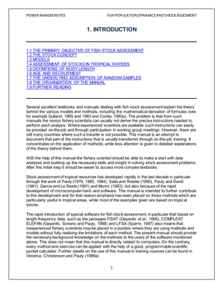
2
1.1 THE PRIMARY OBJECTIVE OF FISH STOCKASSESSMENT
The basic purpose of fish stock assessment is to provide advice on the optimum exploitation of
aquatic living resources such as fish and shrimp. Living resources are limited but renewable,
and fish stock assessment may be described as the search for the exploitation level which in the
long run gives the maximum yield in weight from the fishery.
Fig. 1.1.1 illustrates this basic objective of fish stock assessment. On the horizontal axis is the
fishing effort measured, for example, in number of boat days fished. On the other axis is the
yield, i.e. the landings in weight. (If the landings consist of different groups of animals, for
example shrimp, finfish and squid, it may be more appropriate to express the yield in terms of
value.) It shows that up to a certain level we gain by increasing the fishing effort, but after that
level the renewal of the resource (the reproduction and the body growth) cannot keep pace with
the removal caused by fishing, and a further increase in exploitation level leads to a reduction in
yield.
The fishing effort level which in the long term gives the highest yield is indicated by FMSY and the
corresponding yield is indicated by "MSY", which stands for "Maximum Sustainable Yield". The
phrase "in the long term" is used because one may achieve a high yield in one year by suddenly
increasing the effort, but then meager years will follow, because the resource has been fished
down. Normally, we are not aiming at such single years with maximum yield, but at a fishing
strategy which gives the highest steady yield year after year.
Fig. 1.1.1 The basic objective of fish stock assessment
1.2 THE STOCKCONCEPT

3
When describing the dynamics of an exploited aquatic resource, a fundamental concept is that
of the "stock".
A stock is a sub-set of a "species", which is generally considered as the basic taxonomic unit. A
prerequisite for the identification of stocks is the ability to distinguish between different species.
Because of the great number of different, but often similar, species observed in tropical fisheries
their identification can be problematic. The fishery scientist, however, must master the
techniques of species identification if any meaningful fish stock assessment is to come out of
the data collected. An aid to solve problems in species identification is provided by the "FAO
species identification sheets for fishery purposes" (Fischer, 1978; Fischer and Bianchi, 1984;
Fischer, Bianchi and Scott, 1981; Fischer and Hureau, 1985; Fischer, Schneider and Bauchot,
1987; Fischer and Whitehead, 1974) and in the "FAO species catalogues" (Alien, 1985;
Carpenter, 1988; Carpenter and Alien, 1989; Cohen et al., 1990; Colette and Nauen, 1983;
Compagno, 1984 and 1984a; Holthuis, 1980 and 1990; Márquez, 1990; Nakamura, 1985;
Roper, Sweeney and Nauen, 1984; Russell, 1990; Whitehead, 1985, Whitehead, Nelson and
Wongratana, 1988).
By a "stock" we mean a sub-set of one species having the same growth and mortality
parameters, and inhabiting a particular geographical area.
To this definition we can add that stocks are discrete groups of animals which show little mixing
with the adjacent groups. One essential feature is that the growth and mortality parameters
remain constant over the distribution area of a stock, so that we can use them for making
assessments.
This definition may be too superficial for the taste of many biologists, and in the following
paragraphs a few more aspects of the stock concept are mentioned.
A group of animals for which the geographical limits can be defined may be considered a
"stock" in terms of fish stock assessment. Such a group of animals should belong to the same
race within the species, i.e., share a common gene pool. For species showing little migratory
behaviour (mainly demersal species) it is easier to identify a stock than for highly migratory
species, such as tunas.
A definition of the term "stock" acceptable to everyone with an interest in intraspecific grouping
may be unattainable. For reviews of the stock concept see Booke (1981), Ihssen et al. (1981)
and MacLean and Evans (1981).
Cushing (1968) defines a fish stock as one that has a single spawning ground to which the
adults return year after year. Larkin (1972) defines a stock as "a population of organisms which,
sharing a common gene pool, is sufficiently discrete to warrant consideration as a self-
perpetuating system which can be managed", while Ihssen et al. (1981) define a stock as "an
intraspecific group of randomly mating individuals with temporal or spatial integrity".
Ricker (1975) defines a fish stock as "the part of a fish population which is under consideration
from the point of view of actual or potential utilization". This definition reflects a completely
different approach to the stock concept. In this manual we will not follow this definition at all, but
will adhere to the biological approach given above.

4
Perhaps the most suitable definition in the context of fish stock assessment was given by
Gulland (1983) who stated that for fisheries management purposes the definition of a "unit
stock" is an operational matter, i.e., a sub-group of a species can be treated as a stock if
possible differences within the group and interchanges with other groups can be ignored without
making the conclusions reached invalid.
This means that it is preferable to start by making stock assessments over the entire area of
distribution of a species, as long as there are no indications that separate unit stocks exist in
that area. If it becomes clear that the growth and mortality parameters differ significantly in
various parts of the area of distribution of the species, then it will be necessary to assess the
species on a stock by stock basis. The identification of separate stocks is a complex matter,
which usually requires many years of data collection and analysis.
Fish stock assessment should be made for each stock separately. The results may (or may not)
subsequently be pooled into an assessment of a multispecies fishery. Therefore, the input data
must be available for each stock of each species considered. The stock concept is closely
related to the concepts of growth and mortality parameters. The "growth parameters" are
numerical values in an equation by which we can predict the body size of a fish when it reaches
a certain age. The "mortality parameters" reflect the rate at which the animals die, i.e., the
number of deaths per time unit. The mortality parameters considered in this manual are the
"fishing mortality", which reflects the deaths created by fishing and the "natural mortality", which
accounts for all other causes of death (predation, disease, etc.).
An essential characteristic of a stock is that its growth and mortality parameters remain constant
throughout its area of distribution. Let us, as an example, partition that area into two parts, sub-
areas A and B:
The growth and mortality parameters must be the same in sub-areas A and B, or in other words:
1) The animals in sub-area A must have the same body growth rate as the animals in sub-area
B
2) The animals in sub-area A must have the same probability of death as the animals in sub-
area B
If fishing takes place only in sub-area A, it is assumed that each individual fish in the stock has
the same probability of being encountered in sub-area A and thereby also that it has the same
probability of being caught. The individuals are supposed to move freely between the two sub-
areas.
In order to determine whether a species forms one or more distinct stocks, we should examine
its spawning areas, growth and mortality parameters and morphological and genetic

5
characteristics. We should also compare the fishing patterns in various areas and carry out
tagging studies. The process is complicated, and often it is not possible with the knowledge in
hand to determine whether there are several stocks of that species or not. There are two main
reasons for failing to define a stock properly:
1) The full distribution area of the stock is not covered, so that only a part of the stock is
considered, or the opposite
2) Several independent stocks are lumped together, for example because their areas of
distribution overlap
Several countries may exploit the same stock. This is the case for many migratory stocks, e.g.
tunas. It sometimes happens that a country assesses such a "shared stock" as if it were a
national stock only exploited by that country. On the other hand, a fishery of a single country
may exploit several independent stocks. Coral reef fish stocks may fall in this category.
Fig. 1.2.1 illustrates those two cases. In part I, we consider a fish stock, of which the distribution
area is indicated by a full line. It is exploited by three countries, A, B and C, and we look at the
stock definition from the point of view of the island country C. The broken lines show the EEZ
(Exclusive Economic Zone) of each country, i.e. the national jurisdiction over fisheries. The
dotted area indicates the fishing area of country C and the hatched areas those of countries A
and B. From this it can be seen that if country C would base its assessment on the assumption
that the unit stock is limited to its own fishing area, thus ignoring the fisheries of countries A and
B, it is likely to draw wrong conclusions. If, for example, countries A and B have intensive
fisheries on the stock in question so that it is over-exploited (i.e. a reduction of the fishing
intensity would increase the yield) there is little country C can do on its own to improve the
situation. From the assessment based on the assumption of a stock limited to country C's
waters, country C may conclude that the stock is over-exploited and it may introduce
management measures to reduce fishing. However, the expected effect of the management
measures will not materialize, if countries A and B do not follow country C.
Fig. 1.2.1 Distributions of stocks related to management problems
Part II of Fig. 1.2.1

6
illustrates the case where one fishery exploits several stocks. In this case the assessment
becomes that of the average stock, since it will be impossible to separate the catches by stocks.
If the fishing effort expended is similar for each stock, the result of the assessment should come
out correctly. However, there may also be difficulties in this case. Suppose that the three stocks
currently fished (1, 2 and 3) are heavily overfished, and that the fishery is expanded to include
the unexploited stock 4. In that case the average catch rate will increase and this might lead to
wrong conclusions regarding the status of stocks 1, 2 and 3.
Nearly all exploited marine organisms undertake migrations, for example to their spawning
grounds. A basic key to an understanding of stock structures is the knowledge of migration
routes. This can be obtained from tagging experiments, but also from data and information
provided by the commercial fisheries. Often the fishermen know where the spawning grounds
are and they know where the high concentrations of fish are found at different times of the year.
Some general conclusions may be drawn from the above. Firstly it is usually safer to assume
that species in neighbouring fishing areas form one unit stock than to consider each separate
fishery to exploit its own unit stock. Further, it is evident that proper assessments can only be
carried out when the biology of the species, including its migrations, spawning habits etc., is
fully understood. Fish stocks are not bound by human geographical limits and this means that
proper assessments can only be made when such limits can be ignored through interstate or
international cooperation.
1.3 MODELS
1.3.1 Analytical models
1.3.2 Holistic models
A description of a fishery consists of three basic elements:
1) the input (the fishing effort, e.g. the number of fishing days)
2) the output (the fish landed) and
3) the processes which link input and output (the biological processes and the fishing
operations)
Fish stock assessment aims at describing those processes, the link between input and output
and the tools used for that are called "models". A model is a simplified description of the links
between input data and output data. It consists of a series of instructions on how to perform
calculations and it is constructed on the basis of what we can observe or measure, such as for
example fishing effort and landings.
The actual processes which go from a certain number of days fishing with a certain number of
boats to a certain number of fish being landed are extremely complicated. However, the basic

7
principles are usually well understood, so that by processing the input data by aid of models we
can predict the output.
A model is a good one if it can predict the output with a reasonable precision. However, since it
is a simplification of reality it will rarely (and only by chance) be exact.
The instructions for the calculations that make up the model are given in the form of
mathematical equations. These are composed of three elements: "variables","parameters" and
"operators". For example, the mathematical equation:
y = 2.5 + 3*x
has the variables y and x, the parameters 2.5 and 3 and the operators "+" and "*" The equation
is used to predict the value of y for some value of x.
Fig. 1.3.0.1 General flow-chart for fish stock assessment
Fish stock assessment involves five basic steps as illustrated in Fig. 1.3.0.1. The first step is to
collect data on the fishery, the INPUT to the assessment, which often have to be supplemented

8
by assumptions or qualified guesses. Then we process the data by applying a model to estimate
the growth and mortality parameters, the OUTPUT from the processing of "the historical data".
(The term "historical" is used to distinguish it from the subsequent process, the prediction of
future yield.) This prediction is based on the previous OUTPUT (= INPUT) and on a model, and
the prediction is repeated for a series of alternative options. (Such options could be, for
example, a fishing effort reduction of 10%, 20% and 30%, no change in fishing effort or a fishing
effort increase of 10%, 20% and 30%.) Among the alternative assumptions the best one is
eventually selected as the final OUTPUT. The original INPUT data may be research survey
data, data from samples drawn from the commercial fisheries or a combination of both.
Two main groups of fish stock assessment models are covered in this manual: "holistic models"
and "analytical models". The simple holistic models use fewer population parameters than the
analytical models. They consider a fish stock as a homogeneous biomass and do not take into
account, for example, the length or age-structure of the stock. The analytical models are based
on a more detailed description of the stock and they are more demanding in terms of quality and
quantity of the input data. On the other hand, as a compensation, they are also believed to give
more reliable predictions.
The type of model to be used depends on the quality and quantity of input data. If data are
available for an advanced analytical model then such a model should be used, while the simple
models should be reserved for situations when data are limited. We are often in the situation
where a complete set of input data for an analytical approach is not available, but where the
available data exceed the demand of the simple models. As an alternative to using simple
models in this case, the lacking input data can be replaced by assumptions or qualified
guesswork. Often, the lacking parameter for a particular stock can be replaced by known
parameters from another, similar stock.
1.3.1 Analytical models
A basic feature of analytical models as developed by, among others, Baranov (1914),
Thompson and Bell (1934) and Beverton and Holt (1956), is that they require the age
composition of catches to be known. For example, the number of one year old fish caught, the
number of two year old fish caught, etc. may form the input data.
The basic ideas behind the analytical models may be expressed as follows:
1) If there are "too few old fish" the stock is overfished and the fishing pressure on the stock
should be reduced
2) If there are "very many old fish" the stock is underfished and more fish should be caught in
order to maximize the yield
(Some suggestions for more exact definitions of the term "overfishing" are given in Chapter 8).
The analytical models are "age-structured models" working with concepts such as mortality
rates and individual body growth rates.
The basic concept in age-structured models is that of a "cohort". To put it simply, a "cohort" of
fish is a group of fish all of the same age belonging to the same stock. (We shall further

9
elaborate on the definition of a cohort in Chapter 4.) For example, a cohort of the threadfin
bream, (Nemipterus marginatus) could be all the fish of that species that hatched from June to
August in 1976 near Tanjung Pinang in the South China Sea. Suppose there were one million
specimens in that cohort. After August 1976 the original one million fish would gradually
decrease in number because of deaths due to natural causes (predation, diseases, etc.) or
fishing. However, while the number of survivors of the cohort decreases with time the average
individual body length and body weight increase.
Fig. 1.3.1.1 shows an (hypothetical) example of the dynamics of a cohort, in the form of plots
against age of the number of survivors (A), body length (B), body weight (C) and total biomass
(D). Curve A shows the decay in the number of survivors as a function of the age of the cohort.
Curve B shows how the average body length increases as the cohort grows older. Curve C
shows the corresponding body weight, while curve D is a plot of the total biomass of the cohort,
i.e. the number of survivors times the average body weight against the age of the cohort.
Fig. 1.3.1.1 The dynamics of a cohort

10
Note that curve D has a maximum (at age A1). Thus, to get the (hypothetical) maximum yield in
weight from that cohort all fish should be caught exactly when the cohort has reached age A1.
This, of course, is not possible in practice. However, you may say that the goal of fish stock
assessment is to manage fisheries in such a way that catches come as close as possible to this
theoretical maximum.
The implication is that the fish should neither be caught too young nor too old. If the fish are
caught too young there is "growth overfishing" of the stock.
There are thus two major elements in describing the dynamics of a cohort:
1) The average body growth in length and weight
2) The death process
Both elements will be dealt with in greater detail in Chapters 3 and 4 respectively.
1.3.2 Holistic models
In situations where data are limited, for example, when starting up the exploitation of an hitherto
unexploited resource, or in cases of limited capability of sampling, one may not have input data
of the quality and in the quantity required for an analytical model. One solution would be to start
up the collection of the data types required for the analytical approach and then wait until a
sufficient amount is available. This approach is, of course, recommendable, because it solves
the problem in the long run, but that may take years, while often advice on an exploitation or
development strategy may be needed now. The approach taken in this manual is that no matter
which type of data you have, there is always some information to be extracted from it, and that
advice based on an analysis of a limited data set is usually better than complete guesswork.
In order to cover such data-limited situations, some simple holistic, less data demanding
methods have been included in the manual. These methods disregard many of the details of the
analytical models. They do not use age or length structures in the description of the stocks, but
consider a stock as a homogeneous biomass.
Two types of simple methods are presented, namely the "swept area method" (in Chapter 13)
and the "surplus production model" (in Chapter 9).
The swept area method is based on research trawl survey catches per unit of area. From the
densities of fish observed (the weight of the fish caught in the area swept by the trawl) we obtain
an estimate of the biomass in the sea from which an estimate of the MSY is obtained. This
method is rather imprecise and it predicts only the order of magnitude of MSY.
Fig. 1.3.2.1 Surplus production model

11
The surplus production methods use catch per unit of effort (for example kg of fish caught per
hour trawling) as input. The data usually represent a time series of years and usually stem from
sampling the commercial fishery. The models are based on the assumption that the biomass of
fish in the sea is proportional to the catch per unit of effort as shown in Fig. 1.3.2.1. An estimate
of the yield is obtained by multiplying effort by catch per unit of effort.
1.4 ASSESSMENT OF STOCKSIN TROPICAL WATERS
The literature on fishery biology dealing with species in temperate zones is extensive compared
to that on tropical fisheries. The major part of the literature on tropical fish stock assessment
was published recently. As will appear in the following chapters of the manual, this can partly be
attributed to the fact that tropical resources are somewhat more complex than those of
temperate waters.
The present manual has the word "tropical" in its title. Although the methods described in the
manual resemble those used in temperate waters, there are special features which justify the
use of the word "tropical". Perhaps the most conspicuous difference between fish stock
assessment in tropical waters and temperate waters lies in the nature of the basic input data
rather than in the models.
For the analytical models we need the number of fish caught of each age group as input. In
temperate waters stock assessment methods used are heavily dependent on the fortunate fact
that ages of fish can be readily determined by "ageing" them. Ageing is most often done by
counting rings in hard parts of the fish body, such as ear-bones (otoliths) or scales. The so-
called year-rings are formed through a daily addition (daily-ring) to the size of the scale or
otolith. The chemical composition and thereby the transparency of the addition depends (among
other things) on the amount of food available and is therefore seasonal. The difference in
deposits made in the winter and in the summer can be detected and one year-ring, composed of
a summer and a winter part, can be distinguished from the next. Moreover, temperate fish
species usually spawn once per year in a relatively short time-span, which makes it easy to
distinguish year-classes or cohorts.
Also in tropical fish material is added daily to hard parts, which can be distinguished as daily
growth rings. However, the lack of a strong seasonality makes the distinction of seasonal rings
and therefore also of year-rings problematic for many tropical species. Moreover, the same
absence of strong seasons results in less distinct spawning periods for most species. Many
tropical species spawn at least twice per year and often over long periods. Fortunately, due to
periodic changes in winds (monsoons) and shifts in oceanographic conditions (upwelling) in
many tropical areas, a certain level of seasonality can still be detected. This seasonality may be
reflected in the spawning patterns and growth of tropical fish species albeit less pronounced and
much more difficult to detect than in temperate waters. These seasonal differences make it
possible to detect also in tropical species the existence of different cohorts (often two per year),
through the analyses of length-frequency samples.
In recent years, techniques have been developed to read daily rings in the otoliths of many fish
species. This has enabled the development of age reading on tropical species, in particular of
fish with short life spans, or young fish. These techniques are still very time consuming and will
be difficult to apply on a routine basis. They may however, serve to validate the results obtained
from the analyses of length-frequencies.

12
A further complication of tropical fish stock assessment vis-à-vis that in temperate waters is that
the number of species caught in some important gears, in particular the bottom trawl, is very
high. This does not only affect sampling and data collection procedures, it also makes it more
difficult to apply the models. For a further discussion of differences and similarities between
exploited stocks in arctic, temperate and tropical waters, see Ursin (1984).
The above-mentioned differences can easily explain the slow rate of development of fish stock
assessment in the tropics compared to that in temperate areas. The present manual works with
methods which are the length-based parallels to the traditional age-based methods of temperate
waters.
Clearly, there is a relationship between age and length, and if the relationship is known we can
convert length-frequencies into age frequencies. Fig. 1.4.1 shows a resolution of a length-
frequency sample into age groups (cohorts). There are several techniques available for the
separation of length groups and conversion into age groups, most of which are computerized.
Several of these are discussed in the manual and one of them, the Bhattacharya method, is
illustrated by examples and exercises. This method, although applicable in several
computerized versions, can also be performed by using simply paper, pencil and a (scientific)
pocket calculator.
In this manual, when explaining the theory behind the various methods we often start with the
age-based version, because it is easier to explain and consequently also easier to understand.
The next step is then to convert the age-based method into a length-based method by using the
relationship between age and length.
Fig. 1.4.1 Length-frequencysample resolved into age groups
1.5 DEFINITIONS OF BODY LENGTH
In the present context, "body length" means the average body length of a cohort. Individual fish
are not considered in the models. When talking about "the length of an animal" in connection
with a model it is always tacitly assumed that it is the "average length of the animals of a
cohort". The estimate of average length, however, is derived from averaging the length
measurements of individual specimens. The actual measure used for body length is not
important as far as the theory behind the growth model is concerned. It is common practice to
use the "total length" measured to the "nearest unit below" unless anatomical details make it not
practicable (see Fig. 1.5.1). "Fork length" may be used for fish with stiff caudal fins (tunas) or
special fin shapes (Nemipteridae). The "standard length" is not recommended for length-
frequency sampling.
The most accurate measure for shrimps and lobsters is the "carapace length" (see Fig. 1.5.1).
However, in many cases either total length or tail length is used. In such cases it is necessary to
establish the relationship between the various measurements.
Fig. 1.5.1 Definitions of body length
A really important thing is to specify exactly what kind of length measurement has been used,
as one may otherwise run into difficulties when comparing results with those of other
investigations.

13
Other examples given in Fig. 1.5.1 are squid, octopus, abalone, scallop and sea cucumber. For
animals with a hard shell or skeleton it is not a problem to define a suitable length measure
(fish, crustaceans and molluscs with shell). Also molluscs with a relatively constant body form
(e.g. squid) create no major problem, but animals with a plastic body (e.g. octopus, sea
cucumber or jellyfish) are problematic. It may in certain cases be preferable to work with body
weight rather than length, as the former is obviously measurable with greater accuracy.
It is easy to transform one type of length measurement into another type for a single individual.
In cases where a sample is grouped into length classes it is more cumbersome to change from
one measurement to another as far as the computational aspects are concerned. One simple
way of doing it by microcomputer is given in Sparre (1987).
1.6 AGE AND RECRUITMENT
When working with analytical models we need to define the concept of "age". As was said
above in connection with body length, we do not operate at the individual specimen's level, so
"age" means the average age of a cohort. To define age we must start with a definition of
"birthday". The obvious biological definition of the day of birth is the day the larva hatches from
the egg. We say that a newly hatched fish has age zero.
In the first part of their life the larvae (or juveniles) are usually little influenced by the fishery. We
say that the fish is then in the unexploited phase of life. Because we are interested in the
exploited phase of its life the unexploited phase is not important in the present context.
Let Tr be the youngest age at which the fish may be vulnerable to fishing gears. A fish of age Tr
is called a "recruit". By "recruitment" we mean the number of recruits, i.e. the number of fish that
have attained age Tr during a "recruitment season". The "recruitment intensity" is the number of
recruits per time unit. The "recruitment pattern" of a temperate species could be as shown in
Fig. 1.6.1 A, where each line represents the recruitment intensity in one week. In most tropical
fish stocks recruitment continues (more or less) all year round, but with seasonal oscillations, for
example where monsoons occur (Pauly and Navaluna, 1983) (see Fig. 1.6.1B).
Let us tentatively define the recruitment season of a tropical fish stock by the dates (fractions of
the year) tr1 and tr2 which correspond to the dates of minimum recruitment (see Fig. 1.6.1B).
With 0 < = tr1 < tr2 < = 1.0 we define the "spring cohort" as the fish recruited from time tr1 to tr2
and the "autumn cohort" as the fish recruited from time tr2 to tr1. ("Spring" and "autumn" refer
here to the northern hemisphere).
In general, the recruitment patterns of tropical fish stocks are not very well understood at
present. However, as will appear from the following chapters, the seasonality in recruitment is a
very important prerequisite for the methods suggested.
Fig. 1.6.1 Recruitment intensity during the year of typical temperate and tropical stocks

14

15
1.7 THE UNDERLYING ASSUMPTIONOF RANDOM SAMPLES
All the basic versions of the methods dealt with in the manual assume the input data to be
derived from "random samples". A sample of fish, for example a length-frequency sample
representing the stock, is a random sample if any fish in the entire stock has the same
probability of being drawn as any other.
Usually, it is difficult or even impossible to obtain pure random samples. If, for example, the
juvenile fish are located in certain nursery areas, which do not coincide with the fishing grounds
from which our samples originate, the juvenile fish will be under-represented in the samples. A
similar problem is created by the selectivity of fishing gears. Often the small fish are under-
represented because they escape through the meshes, whereas the larger fish are retained.
Samples which are not random samples are called "biased samples".
A feature of fish behaviour which is believed to create the most serious bias is
"migration". Almost all marine animals perform systematic movements. Pelagic fish such as
mackerels, scads and tunas undertake long migrations between feeding grounds and spawning
grounds. Most penaeid shrimps start their life cycle in the open sea and migrate to shallow
waters (lagoons and mangroves) and when sexually mature they migrate back to the open sea
for reproduction.
The implication of the migratory behaviour is that a large sea area must be covered in order to
obtain random samples from the entire population. Often samples can be obtained only from the
commercial fishery which concentrates on those grounds where the resources are easiest to
catch in large quantities. Thus, we are often in the situation that random samples of the
population are not available. This bias must be accounted for in the analysis and the basic
methods have to be modified to account for it. Some types of bias are easier to deal with than
others. Bias created by migration can only be handled properly when the migration routes are
known. When they are not we have to make certain assumptions about them in order to get on
with the analysis. There are many serious problems in connection with bias. A few suggestions
on how to get around them are presented, but the manual also leaves a number of relevant
questions open, either because the author does not know the answer or the method is so
complicated that it falls outside the scope of this manual. Unfortunately, one often comes across
cases in practice, which are so heavily influenced by bias that they cannot be handled by the
methods described here (see Chapter 11).
1.8 THE ORGANIZATION OF THE MANUAL
The complexity of fish stock assessment is reflected in the contents table of this manual. The
various elements cannot be dealt with simultaneously and it has often been necessary to refer
to earlier or later sections and chapters. In order to assist the reader (and teacher) a flowchart
for fish stock assessment as presented in this manual is given in Fig. 1.8.1. The flowchart does
not present the methods in the same sequence as they appear in the manual, but rather in the
natural chronological order of a fish stock assessment. The numbers of the relevant chapters
are given in brackets.
Before starting as a fish stock assessment worker there are a few general basic statistical
techniques (for example linear regression analysis) one must master. These are dealt with in
Chapter 2. They have been placed outside the proper flow-chart, because the methods are

16
general and applied in many other scientific fields. Chapter 2 contains only a small selection of
statistical methods and only those which are needed to follow the text in the subsequent
chapters.
The flow-chart is divided into two parts. Part A deals with analytical methods and Part B deals
with holistic methods. As the sizes of the two parts indicate, the main emphasis has been
placed on the analytical methods. Both approaches follow the same main lines, namely the set-
up given in Fig. 1.3.0.1.
Part A, the analytical methods
The first row shows the input to the estimation of growth parameters (the parameters by which
we can predict the length of an animal for a given age). Although collection of data comes first
chronologically, it is not dealt with in the beginning of the manual, because one cannot deal with
data collection in a meaningful way before the objectives of the sampling scheme have been
defined. To define the objectives we need the models used for the analysis of historical data,
therefore, the main text on data collection is deferred to Chapter 7. The assumptions indicated
as input are not dealt with in a particular chapter.
The theory behind the model for body growth and the estimation of growth parameters is dealt
with in Chapter 3. Handling of bias problems is as mentioned above extremely complicated and
only partly covered by the present manual. It has therefore been placed in Chapter 11 after the
chapters dealing with the analytical methods in their basic versions.
Fig 1.8.1A The organization of the manual
Fig. 1.8.1B The organization of the manual
Although we should start the analysis with an evaluation of the bias, it has not been considered
appropriate to start the manual with one of the most complicated subjects. Also the estimation
or rather the qualified guessing on natural mortality is a tricky subject. It has been placed in
Section 4.7.
The following chapters on analytical methods contain the theory for both age-based methods
and length-based methods. The estimates of growth parameters are in fact only used for the
length-based versions of the models, but in order to reduce the complexity of the flow-chart, no
distinction has been made between length-based and age-based methods.
After the growth part (Chapter 3) the flow-chart branches. The two branches represent a
grouping of methods according to their data requirements. Some analytical methods are based
exclusively on samples from the commercial fishery, while the total catch is not known. In
theory these methods could be used also on a single sample consisting of one bucket of fish
sampled in the local fish market (although, of course, extensive sampling schemes are
recommended). Such methods are called "catch curve methods".
Other methods are based on estimates of the total catch, i.e. on estimates of the total number
landed in each length group from the entire stock. Such numbers are derived from length-
frequency samples by raising them to account for the entire catch using data on total landings.
These methods are called "cohort analysis" or "Virtual Population Analysis" (VPA). Compared to
the catch curve methods, they give more dependable estimates of the parameters and more

17
reliable predictions of the future fishery. The sampling procedures to obtain the input data are
discussed in Chapter 7 as mentioned above in connection with growth.
The general theory of the death process, the "exponential decay model", the "catch curve
methods" and some other methods with similar or limited data requirements is dealt with in
Chapter 4. From the catch curve analysis we obtain an estimate of the total mortality, which
combined with growth parameters and natural mortality, allows us to arrive at some conclusions
on the current state of the stock and its potential. This analysis is performed by the "Beverton
and Holt yield per recruit model", which is presented in Chapter 8. The ultimate result is the
"maximum sustainable yield per recruit" (MSY/R).
The methods based on the size composition of the total catch, the cohort analysis and the VPA
are covered in Chapter 5. The results obtained from cohort analysis (or VPA) are estimates of
absolute stock size and fishing mortality for each size group. These results are used for the
prediction of stock biomass and yield levels using the "Thompson and Bell methods" which are
described in Chapter 8. The final result is an estimate of the (absolute) MSY.
In the discussion presented above only the regulation of fishing effort has been considered as
an instrument for fisheries management. However, there are other instruments, one of which is
the size selectivity of the fishing gear. For example, by using larger mesh sizes in the codend of
a trawl, the mortality on young fish is reduced, which subsequently will increase the catch of
older, larger and more valuable specimens. The effects of "gear selectivity" are discussed in
Chapter 6.
In all the chapters mentioned so far, the theory has been presented in its most simple form, i.e.
only one stock of fish and only one type of fishing boat are considered. In reality there hardly
exists any fishery where only one species is caught by only one type of boat. In most cases we
have to deal with multispecies catches made by a variety of different boats. In theory it does not
create any major problems to extend the analytical models to deal with the
multispecies/multifleet case, and this has been demonstrated for the Thompson and Bell model
in Chapter 10. Some other aspects of multispecies assessment are also briefly discussed in this
chapter. With this we have reached the end of Part A of the flow-chart.
Part B, the holistic methods
This part of the flow-chart is less complicated, because it describes simpler methods. The
"surplus production models" are presented in Chapter 9 and the "swept area method" in
Chapter 13.
Chapters 12, 14 and 15 have not been included in the flow-chart. Chapter 12 deals with the
stock/recruitment relationship - the question of a possible relationship between recruitment and
the size of the parent stock. The problem is discussed in essay form and Chapter 12 does not
suggest any models for practical application. Chapter 14 provides an overview of fish stock
assessment, based among other things on the same flow-chart (Fig. 1.8.1). Chapter 15
describes briefly some microcomputer program packages, the LFSA (Length-based Fish Stock
Assessment) package (Sparre, 1987), which matches the analytical models of this manual (Part
A of the flow-chart), the COMPLEAT ELEFAN package (Gayanilo, Soriano and Pauly, 1988)
and the FiSAT (FAO/ICLARM Stock Assessment Tools) package (in press) which also covers
all the models. Some other programs developed by or in close cooperation with FAO have also
been briefly described.

18
1.9 FURTHER READING
Since the scope of this manual is mainly limited to methods and their applications, it is advisable
to supplement the knowledge derived from it, by reading additional textbooks and manuals on
stock assessment and on the biology of the most important resources. Chapter 16 contains
references to several recent publications, which will be of great use in providing a better insight
to stock assessment problems, for example
1) The relationship between stock assessment and management (Pauly, 1979 and Gulland,
1988)
2) The biology and assessment of shrimps (Garcia and Le Reste, 1981; Gulland and Rothschild,
1984; Penn, 1984; Garcia, 1985; Rothlisberg, Hill and Staples, 1985, the Australian Journal of
Marine and Freshwater Research, 1987 and Dall et al., 1990)
3) The biology and assessment of cephalopods and other invertebrates (Caddy, 1983, 1983a
and 1989)
4) Resource mapping (Caddy and Garcia, 1986 and Butler et al., 1986)
5) Tunas (Sharp and Dizon, 1978; Kleiber, Argue and Kearney, 1983; I-ATTC, 1984 and
Hunter et al., 1986)
6) Migration (Harden Jones, 1968, 1984 and Oxenford and Hunte, 1986)
7) Marine population regulation and speciation (Sinclair, 1988)
The various methods presented in this manual were used either directly or through the LFSA
and COMPLEAT ELEFAN packages at FAO/DANIDA follow-up training courses, where
participants processed their own data. The results of the analyses and the input data were
published (Venema, Christensen and Pauly, 1988), with the aim of providing additional
examples of the application of stock assessment methods on tropical resources. In some cases
the papers demonstrate clearly the limitations of the data sets and of the methods used, but
there are also several examples of successful applications of methods hitherto seldom used in
tropical areas.
New text books on fish stock assessment are rare, and we are therefore pleased to draw your
attention to recent books by Hilborn and Walters (1992) and Brêthes and O'Boyle (eds.) (1990).
The latter is partly based on an earlier version of this manual.
A comprehensive overview of the several approaches on the use of length-frequency data for
stock assessment purposes was prepared by J.A. Gulland and A.A. Rosenberg (1992). This
document, John Gulland's last contribution to fisheries science, should be used in conjunction
with or as a follow-up to this manual.

Fish population dynamics and shock assesment(5th sem)

Recommandé

Recommandé

Contenu connexe

Tendances

Tendances (20)

Similaire à Fish population dynamics and shock assesment(5th sem)

Similaire à Fish population dynamics and shock assesment(5th sem) (20)

Plus de SHUBHAM PATIDAR FISHERIES ADDAA

Plus de SHUBHAM PATIDAR FISHERIES ADDAA (20)

Dernier

Dernier (20)

Fish population dynamics and shock assesment(5th sem)