Individuals with abnormal walking patterns due to various conditions face significant challenges in daily activities, especially walking. Ankle-foot orthosis (AFO) devices are crucial in providing essential support to their lower limbs. Accurately modeling the dynamic behavior of AFO systems, particularly in predicting ground reaction forces, is a complex yet vital task to ensure their effectiveness. This research develops dynamic models for AFO systems using advanced modeling techniques, employing both parametric and non-parametric approaches. Parametric methods, such as particle swarm optimization (PSO), and non-parametric methods, like multi-layer perceptron (MLP) neural networks, are utilized through system identification methods. According to the findings, the MLP neural network continuously generates objective results and performs exceptionally well in correctly detecting the AFO system, attaining a noticeably lower mean squared prediction error of 0.000011. This research highlights the potential of advanced modeling techniques, particularly MLP neural networks, in enhancing AFO system modeling accuracy. Although parametric techniques like PSO are useful, the MLP approach performs better, offering insightful information about modelling AFO systems and indicating that non-parametric techniques like MLP neural networks have potential to further AFO creation and control.

1. TELKOMNIKA Telecommunication Computing Electronics and Control
Vol. 23, No. 2, April 2025, pp. 484~494
ISSN: 1693-6930, DOI: 10.12928/TELKOMNIKA.v23i2.25876  484
Journal homepage: http://telkomnika.uad.ac.id
Imposing neural networks and PSO optimization in the quest
for optimal ankle-foot orthosis dynamic modelling
Annisa Jamali1
, Aida Suriana Abdul Razak1
, Shahrol Mohamaddan2
1
Department of Mechanical Engineering, Faculty of Engineering, Universiti Malaysia Sarawak, Sarawak, Malaysia
2
College of Engineering, Shibaura Institute of Technology, Tokyo, Japan
Article Info ABSTRACT
Article history:
Received Nov 21, 2023
Revised Nov 28, 2024
Accepted Dec 26, 2024
Individuals with abnormal walking patterns due to various conditions face
significant challenges in daily activities, especially walking. Ankle-foot
orthosis (AFO) devices are crucial in providing essential support to their lower
limbs. Accurately modeling the dynamic behavior of AFO systems,
particularly in predicting ground reaction forces, is a complex yet vital task to
ensure their effectiveness. This research develops dynamic models for AFO
systems using advanced modeling techniques, employing both parametric and
non-parametric approaches. Parametric methods, such as particle swarm
optimization (PSO), and non-parametric methods, like multi-layer perceptron
(MLP) neural networks, are utilized through system identification methods.
According to the findings, the MLP neural network continuously generates
objective results and performs exceptionally well in correctly detecting the
AFO system, attaining a noticeably lower mean squared prediction error of
0.000011. This research highlights the potential of advanced modeling
techniques, particularly MLP neural networks, in enhancing AFO system
modeling accuracy. Although parametric techniques like PSO are useful, the
MLP approach performs better, offering insightful information about
modelling AFO systems and indicating that non-parametric techniques like
MLP neural networks have potential to further AFO creation and control.
Keywords:
Ankle-foot orthosis
Modeling
Neural network
Particle swarm optimization
System identification
This is an open access article under the CC BY-SA license.
Corresponding Author:
Annisa Jamali
Department of Mechanical Engineering, Faculty of Engineering, Universiti Malaysia Sarawak
Sarawak, Malaysia
Email: jannisa@unimas.my
1. INTRODUCTION
The medical condition known as a stroke happens when the brain’s blood supply is interrupted,
harming brain nerves and interfering with information transmission between the brain and the limbs [1]. One
consequence of stroke can be foot drop, a neuromuscular disorder [2]. When walking in the swing phase,
patients with foot drops drag their toes because they have difficulty dorsiflexing their feet [3]-[6].
As seen in Figure 1, these patients consequently exhibit variations from the typical gait pattern. Ankle-
foot orthoses (AFOs) are frequently utilised for rehabilitation training in this situation since they offer stability
and preserve range of motion. AFOs have been shown to increase gait speed when compared to non-AFO
scenarios [7]-[9]. This improvement in gait velocity is important because it directly affects the quality of life
for stroke survivors, allowing them to move more efficiently and reduce the risk. To ensure that patients receive
the most advantages, clinicians must thus understand the mechanical properties of AFOs, such as rigidity and
their effects on gait [10]-[13]. It is of the utmost importance, in clinical practice, to modify the torque of AFO
in accordance with the unique body function and gait capabilities of each patient [14], [15]. Nevertheless,

2. TELKOMNIKA Telecommun Comput El Control 
Imposing neural networks and PSO optimization in the quest for optimal ankle-foot … (Annisa Jamali)
485
conventional therapeutic approaches that rely on manual support are laborious for practitioners and could not
offer continuous assistance for prolonged durations [16], [17].
Figure 1. Walking gait phase; initial contact (IC), foot flat (FF), heel-off (HO), and toe-off (TO) [12]
Modeling AFO is challenging, particularly when considering ground reaction forces in complex
systems with multiple points of ground contact [18]. AFO models have been created using a variety of
techniques, such as musculoskeletal simulations, direct multiple shooting techniques, Monte Carlo simulations,
computational modelling and functional electrical stimulations [19], [20]. In recent years, system identification
has gained attention for accurately modeling dynamic systems. Parametric identification involves two phases:
qualitative operation, which establishes the system’s structure, and identification, which determines numerical
values for structural parameters. Traditional methods like the least squares method and Zatsiorsky regression
equations have been used for parametric identification [21]. The goal is to apply this control method’s inverse
dynamic model to human gait systems.
While genetic algorithms are well-known as a stochastically optimal approach, particle swarm
optimization (PSO), another global optimization algorithm, has gained prominence [22]. PSO relies on social
information exchange among members of a group to find specific parameter sets that optimize an objective
function. It is suitable for nonlinear design spaces with discontinuities and diverse constraints.
Non-parametric models often incorporate components of soft computing methods, such as neural
networks (NNs) and fuzzy logic. Deep neural networks consist of layers of artificial neurons that mimic
biological neurons’ functioning, making them effective for various machine learning tasks. Decision trees,
utilized in random forests, contribute to the final classification by aggregating judgments based on input
variables. Research indicates that deep neural network models perform well, particularly in predicting the need
for AFOs [23].
The aim of this research is to explore the performance of the dynamic model for AFO using parametric
and non-parametric modelling methodologies. The parametric approach involves the utilization of PSO, while
the non-parametric approach employs multi-layer perceptron (MLP) neural networks. These models are created
using information obtained from an experimental setup and the system identification approach. Following
model development, a thorough validation process ensues, with the acquired results subject to meticulous
comparison and analysis. The findings provide to improving the development and control of AFO systems,
benefiting individuals with mobility impairments caused by conditions like foot drop, stroke, and other
disabilities.
2. METHOD
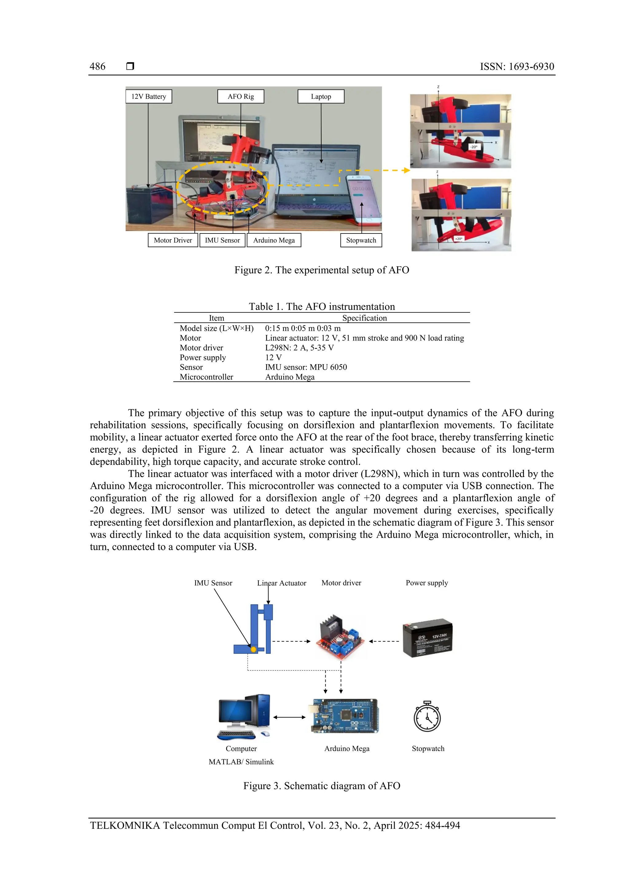
This study presents a comprehensive approach to modeling an AFO, as illustrated in Figure 2. The
proposed algorithm is designed to accurately replicate the dynamic behavior of the ankle. By incorporating
both parametric and non-parametric techniques, the study explores various modeling options to identify the
most effective approach. Ultimately, this modeling framework aims to enhance the development and control
of AFOs, ensuring they closely mimic the natural dynamics of the ankle.
2.1. Experimentation set up and data acquisition
Initially, an AFO rig with one degree of freedom (DOF) was designed and fabricated. The structure
specifically designed for children utilized 3D printing materials, boasting approximate dimensions of
0.15 m × 0.05 m × 0.03 m. Table 1 outlines the specifications of the instrumentation employed in this study.

3.  ISSN: 1693-6930
TELKOMNIKA Telecommun Comput El Control, Vol. 23, No. 2, April 2025: 484-494
486
Figure 2. The experimental setup of AFO
Table 1. The AFO instrumentation
Item Specification
Model size (L×W×H) 0:15 m 0:05 m 0:03 m
Motor Linear actuator: 12 V, 51 mm stroke and 900 N load rating
Motor driver L298N: 2 A, 5-35 V
Power supply 12 V
Sensor IMU sensor: MPU 6050
Microcontroller Arduino Mega
The primary objective of this setup was to capture the input-output dynamics of the AFO during
rehabilitation sessions, specifically focusing on dorsiflexion and plantarflexion movements. To facilitate
mobility, a linear actuator exerted force onto the AFO at the rear of the foot brace, thereby transferring kinetic
energy, as depicted in Figure 2. A linear actuator was specifically chosen because of its long-term
dependability, high torque capacity, and accurate stroke control.
The linear actuator was interfaced with a motor driver (L298N), which in turn was controlled by the
Arduino Mega microcontroller. This microcontroller was connected to a computer via USB connection. The
configuration of the rig allowed for a dorsiflexion angle of +20 degrees and a plantarflexion angle of
-20 degrees. IMU sensor was utilized to detect the angular movement during exercises, specifically
representing feet dorsiflexion and plantarflexion, as depicted in the schematic diagram of Figure 3. This sensor
was directly linked to the data acquisition system, comprising the Arduino Mega microcontroller, which, in
turn, connected to a computer via USB.
Figure 3. Schematic diagram of AFO
12V Battery AFO Rig Laptop
Motor Driver Arduino Mega Stopwatch
IMU Sensor
IMU Sensor Linear Actuator Motor driver Power supply
Computer
MATLAB/ Simulink
Arduino Mega Stopwatch

4. TELKOMNIKA Telecommun Comput El Control 
Imposing neural networks and PSO optimization in the quest for optimal ankle-foot … (Annisa Jamali)
487
A personal notebook with a powerful processor, 4.00 GB of RAM, and MATLAB software was used
to analyse the generated signals. The Simulink program was used to create the interface for data gathering. An
other technique was to apply a bang-bang torque signal to the AFO in order to simultaneously activate the
actuator with the required torque.
2.2. System identification
The dynamic system of the AFO was modelled in this work using the system identification technique.
In this technique, four main stages were involved that is data acquisition, model structure selection, model
estimation, and model validation. To explore the effects of parametric and non-parametric approaches, the
model estimation in this study was conducted using PSO and MLPNN, respectively. Subsequently, system
identifications were formulated utilizing an auto-regressive with exogenous (ARX) and nonlinear auto-regressive
with exogenous (NARX) model structure, correspondingly. The ARX model structure is describe in (1):
𝑦(𝑡) =
𝐵(𝑧−1)
𝐴(𝑧−1)
𝑢(𝑡) +
𝜀(𝑡)
𝐴(𝑧−1)
(1)
where the expressions of A(z−1) and B(z−1) are;
𝐴(𝑧−1) = 1 + 𝑎1𝑧−1
+ … . + 𝑎𝑛𝑧−𝑛
(𝑧−1) = 𝑏0 + 𝑏1𝑧−1
+ … . + 𝑏𝑛𝑧−(𝑛−1)
(2)
White noise, 𝜀(𝑡)=0, n is the model’s orders, and [𝑎1, … , 𝑎𝑛, 𝑏1, … , 𝑏𝑛] are the model parameters that need to
be estimated to determine 𝑧−1
. The system’s output vector is denoted by 𝑦(𝑡) and its input vector by 𝑢(𝑡). In
(3) yields the neural network auto regressive model with eXogenous inputs (NNARX) model structure
regression vector. Through the integration of neural networks into the model framework, NNARX overcomes
the drawbacks of NARX.
𝜑(𝑡) = [𝑦(𝑡 − 1), … . , 𝑦(𝑡 − 𝑛𝑎,), 𝑢(𝑡 − 𝑘), … . , 𝑢(𝑡 − 𝑛𝑏 − 𝑛𝑘 + 1)]𝑇
(3)
where 𝜑(𝑡) denotes the regression vector at time step, t. Past values of the system’s input and output are used
to generate the regression vector. In (4) gives the one step ahead (OSA) forecast of the NNARX model:
𝑦
̂ (
𝑡
𝜃
) = 𝑦 (
𝑡
𝑡−1
, 𝜃) = g (𝜑(𝑡), 𝜃) (4)
where g is the function that the neural network approach has achieved.
2.2.1. Parametric estimation via particle swarm optimization
Parametric system identification involves utilizing measurable data to develop mathematical models
that represent a dynamic system [24]. Good models are necessary for most model-based control methods. The
key task after defining the model structure is to estimate its parameters, typically determined by applying a
global minimum criterion function. PSO was inspired by the study of natural social behaviors in animals, such
as schools of fish, swarms of bees, and bird flocks, and operates based on a population model [25]. PSO is easy
to apply to a variety of optimisation issues and has a straightforward approach. Although it can be challenging
to initialise its parameters. Despite the fact that initialising its parameters can be difficult, PSO has a high
chance and efficiency of finding the global optima and requires few modifications. PSO can converge too
quickly and get stuck in local optima, despite its quick error convergence.
In the process of identifying the optimal solution in multidimensional space, the PSO algorithm
mimics birds using N particles [26]. Position (𝑃𝑖) and velocity (𝑉𝑖), where i is the particle label, are the two
characteristics of every particle. The particle’s movement is represented by (𝑉𝑖), as seen in (5). (𝑃𝑖) is the
outcome of the particle’s motion and a potential solution to the associated optimisation problem, as illustrated
in (6). Each particle’s fitness value 𝐹𝑖, which is calculated using mean squared error (MSE), quantifies the
difference between the current candidate solution and the best solution. The individual extremum 𝐺𝑖 is the
optimal solution for individual particle search, in contrast to its historical and present solutions. For the whole
particle swarm, the population extremum Z is the best solution relative to its historical solution and all
individual extremum of the current generation. The particle population continuously updates the position and
velocity of particles by monitoring both individual and group extremums during the search and iteration process
in order to identify the optimal solution that satisfies the requirements. The optimisation outcome can be seen
in the final group extremum Z.

5.  ISSN: 1693-6930
TELKOMNIKA Telecommun Comput El Control, Vol. 23, No. 2, April 2025: 484-494
488
𝑉𝑖−𝑛𝑒𝑤 = 𝜔𝑉𝑖 + 𝑐1𝑟𝑎𝑛𝑑()(𝐺𝑖 − 𝑃𝑖) + 𝑐2𝑟𝑎𝑛𝑑()(𝑍 − 𝑃𝑖) (5)
𝑉𝑖−𝑛𝑒𝑤 = 𝑉𝑖 + 𝑃𝑖 (6)
where the left part of the equation represents the new velocity and position of the particle in the current
generation, and the right part represents the particle properties from the previous generation. The inertia factor
𝜔 is equal to 0.5. 𝑐1 and 𝑐2 are learning factors with values of 2. In addition, the population size N (1,599) was
adjusted to N/2, resulting in 799.5 and the maximum number of iterations M was set to 1,000.
2.2.2. Non-parametric estimation by using multi-layer perceptron neural network
The AFO was modelled using an MLP neural network for non-parametric estimation. The MLP neural
network family is the most commonly utilised because it can estimate a very complex formula association
while producing a simple model [27]. In the MLP, the input layer is formed by a single set of nodes, and the
output is generated by a second layer, with several hidden layers positioned between them. The input layer 𝑥𝑖,
output layer 𝑦𝑗, and hidden layer 𝑤𝑖𝑗 with different strength weights make up the network layer. The qualities
of the function 𝑓(. ) include radial basis, hyperbolic tangent, sigmoid, threshold, and linear. The network can
forecast the output, 𝑦
̂, as precisely as feasible thanks to the mapping. In (7), the MLP output is displayed:
𝑦
̂(𝑤, 𝑊) = 𝐹𝑖(∑ 𝑊𝑖𝑗 ∙
𝑞
𝑗=1 𝑓𝑗(∑ 𝑤𝑖𝑗𝑋𝑖 +
𝑚
𝑖=1 𝑤𝑗0) + 𝑊𝑖0) (7)
Levenberg-Marquardt (LM) is chosen for training networks because of its fast convergence, even
though it demands higher memory usage compared to alternative algorithms. The LM minimises the residual,
𝜀(𝑡, 𝜃) = 𝑦(𝑡) − 𝑦
̂(𝑡, 𝜃), in order to maximise the error based on the criterion in (8):
𝐿𝑖
(𝜃) = (
1
2𝑁
) ∑ 𝜀−2
(𝑡, 𝜃) ≈
𝑁
𝑡=1 𝑃𝑁(𝜃, 𝑍𝑁
) (8)
where 𝑍𝑁
represents the training data set.
2.2.3. Model validation
To ensure the adequacy of the model under development, the validation phase is essential [15]. This
validation process employs three methods: OSA prediction, MSE, and correlation test. The study examines
five correlation functions:
𝜑𝜀𝜀(𝜏) = 𝐸[𝜀(𝑡 − 𝜏)𝜀(𝑡)] = 𝛿(𝜏),
𝜑𝑢𝜀(𝜏) = 𝐸[𝑢(𝑡 − 𝜏)𝜀(𝑡)] = 0, ∀𝜏,
𝜑𝜀2𝜀(𝜏) = 𝐸[𝑢2(𝑡 − 𝜏) − 𝑢
̅2
(𝑡)𝜀(𝑡)] = 0, ∀𝜏, (9)
𝜑𝜀2𝜀2(𝜏) = 𝐸[𝑢2(𝑡 − 𝜏) − 𝑢
̅2
(𝑡)𝜀2
(𝑡)] = 0, ∀𝜏,
𝜑𝜀(𝜀𝑢)(𝜏) = 𝐸[𝜀(𝑡)𝜀(𝑡 − 1 − 𝜏)𝑢(𝑡 − 1 − 𝜏)] = 0, 𝜏 ≥ 0,
𝜀𝑢(𝑡) = 𝜀(𝑡 + 1)𝑢(𝑡 + 1), 𝛿(𝜏) is an impulse function, and 𝜑𝑢𝜀(𝜏) is the cross-correlation function
between 𝑢(𝑡) and 𝜀(𝑡). All five requirements need to be met because the MLP model is built using the NARX
structure, which makes it a nonlinear system. Conversely, another PSO model employing a linear system
necessitates the fulfillment of only three conditions.
The study employs 1,599 data points for PSO and 2,189 data points for MLP in testing. The selection
of 1,599 data points for PSO aims for increased stability in results, while 2,189 data points for MLP correspond
to the entirety of five walking cycles during the experiment. The 95% confidence bands are used, which are
around ±1.96/√N (N data), with one or more function points falling outside of these limits indicating a
substantial link [28]. The model is deemed adequate if the correlation functions remain within the confidence
intervals.
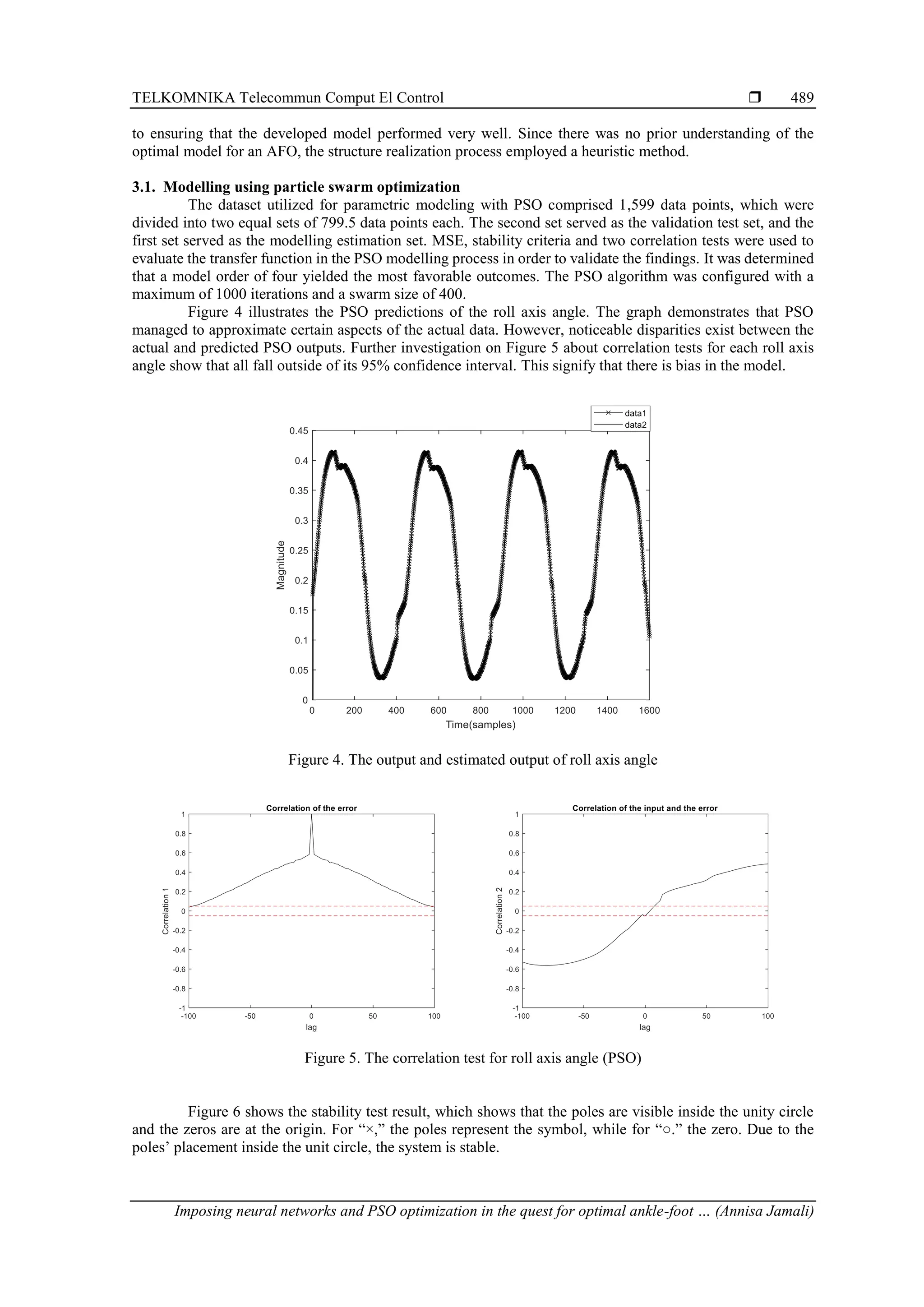
3. RESULTS AND DISCUSSION
In this research, the collected datasets were split into two parts: one for training the model and the
other for evaluating its performance. The validation of the developed system involved multiple metrics,
including MSE, OSA prediction, correlation tests, and examination of the pole-zero diagram for stability.
The most appropriate model was chosen primarily based on robustness studies, with an emphasis on
achieving a low MSE, high stability, and unbiased outcomes in correlation tests. These evaluations were critical

6. TELKOMNIKA Telecommun Comput El Control 
Imposing neural networks and PSO optimization in the quest for optimal ankle-foot … (Annisa Jamali)
489
to ensuring that the developed model performed very well. Since there was no prior understanding of the
optimal model for an AFO, the structure realization process employed a heuristic method.
3.1. Modelling using particle swarm optimization
The dataset utilized for parametric modeling with PSO comprised 1,599 data points, which were
divided into two equal sets of 799.5 data points each. The second set served as the validation test set, and the
first set served as the modelling estimation set. MSE, stability criteria and two correlation tests were used to
evaluate the transfer function in the PSO modelling process in order to validate the findings. It was determined
that a model order of four yielded the most favorable outcomes. The PSO algorithm was configured with a
maximum of 1000 iterations and a swarm size of 400.
Figure 4 illustrates the PSO predictions of the roll axis angle. The graph demonstrates that PSO
managed to approximate certain aspects of the actual data. However, noticeable disparities exist between the
actual and predicted PSO outputs. Further investigation on Figure 5 about correlation tests for each roll axis
angle show that all fall outside of its 95% confidence interval. This signify that there is bias in the model.
Figure 4. The output and estimated output of roll axis angle
Figure 5. The correlation test for roll axis angle (PSO)
Figure 6 shows the stability test result, which shows that the poles are visible inside the unity circle
and the zeros are at the origin. For “×,” the poles represent the symbol, while for “○.” the zero. Due to the
poles’ placement inside the unit circle, the system is stable.

7.  ISSN: 1693-6930
TELKOMNIKA Telecommun Comput El Control, Vol. 23, No. 2, April 2025: 484-494
490
Figure 6. The stability test for roll axis angle (PSO)
Table 2 presents the numerical outcomes of the optimal model order. It is noteworthy that each model
demonstrates bias, prompting the utilization of MSE values as indicators for determining the superior model.
Among the various model orders evaluated, it was found that model order 4 yielded the lowest MSE values for
both the training and testing datasets, which were 1.8075×10-4 and 1.7743×10-5, respectively, thus
establishing it as the optimal model for PSO optimization method.
Table 2. Comparison of PSO optimization performance in different number of model order
Model order MSE in training data MSE in testing data Stability Correlation test
2 1.3612×10-4
6.1793×10-5
Unstable Biased
4 1.8075×10-4
1.7743×10-5
Stable Biased
6 2.6758×10-4
1.2621×10-5
Stable Biased
8 4.4309×10-4
8.9236×10-5
Unstable Biased
10 9.7826×10-4
5.2718×10-4
Unstable Biased
3.2. Modelling using multi-layer perceptron
The dataset comprising 2,189 data points for non-parametric modeling with neural network multi-
layer perceptron (NN MLP) was split into two sets: one containing 1,532 points for modeling (the estimation
set) and the other containing 657 points for validation (the test set). To validate the results, the NN MLP
modeling was compared using MSE and five correlation tests. Given the lack of prior knowledge regarding
appropriate delay numbers and model structures for NN MLP, a heuristic method was employed to determine
the structure.
During this technique, three crucial factors were considered: the error, the size of the NN structure (or
the number of neurones), and the number of delay signalsDue to the randomness involved in selecting the best
model, assessing the final component was crucial in determining the ideal number of delay signals and the
configuration for each model. Validation MSE, modelling MSE, and correlation tests were used to determine
the selection criteria.
The study started with a model structure of [2 2 1], which included one neurone in the output layer,
two neurones in the second hidden layer, and two neurones in the first hidden layer. The delay number served
as a representation of the input layer. Eight delay signals, eight neurones in the first and second hidden layers,
and one neurone in the output layer were then used to improve model performance, resulting in a model
structure of [8 8 1]. Figure 7 shows the MLP predictions for the roll axis angle, with the actual data shown by
a vertical line at point 1,532. With a nearly zero difference between the real and anticipated MLP output, the
graph shows how well the MLP tracks the actual data.

8. TELKOMNIKA Telecommun Comput El Control 
Imposing neural networks and PSO optimization in the quest for optimal ankle-foot … (Annisa Jamali)
491
Figure 8 shows the correlation test results for all roll axis angles. The accurateness of the model is
demonstrated by the MLP results, which clearly lie inside the 95% confidence level. This underscores the
unbiased nature of the model’s predictions. Table 3 displays the numerical results pertaining to the optimal
model structure and delay of NN MLP. Among the listed configurations, the model structure [8 8 1] with 8
delays stands out, showcasing the lowest MSE of 1.1034×10-5
, thus confirming its status as the best-performing
model.
Figure 7. The output and estimated output of roll axis angle (MLP)
Figure 8. The correlation test for roll axis angle (MLP)

9.  ISSN: 1693-6930
TELKOMNIKA Telecommun Comput El Control, Vol. 23, No. 2, April 2025: 484-494
492
Table 3. Comparison of NN MLP performance
Model structure Delay MSE Correlation test
[2 2 1] 2 2.3829×10-4
Unbiased
[4 4 1] 2 3.5671×10-4
Unbiased
[6 6 1] 6 2.7149×10-4
Unbiased
[8 8 1] 7 1.8625×10-4
Unbiased
[8 8 1] 8 1.1034×10-5
Unbiased
3.3. Comparative assessment and discussion
Thorough training and testing protocols, together with extensive correlation studies, have been used
to validate PSO and NN MLP-based models. The outcomes of these assessments consistently show that the
different modelling approaches taken into consideration in this study function satisfactorily. With an emphasis
on mean-squared error and correlation test results, Table 3 provides a succinct overview of the relative
effectiveness of parametric and non-parametric modelling techniques.
When comparing the performance of the two modelling methodologies, Table 4 demonstrates that the
NN MLP-based non-parametric approach offers a better approximation to the system response than PSO. This
conclusion is consistent with earlier studies showing that parametric modelling techniques like GA typically
produce inferior results versus non-parametric techniques like NN MLP [13]. Additionally, the results of the
correlation test show that NN MLP performs better than PSO, showing a smaller mean-squared error.
Table 4. Performance of parametric and non-parametric modelling approaches
Algorithm MSE Correlation test
NN MLP 0.000011034 Unbiased
PSO 0.00018075 Biased
However, a notable advantage of PSO lies in its fewer parameters requiring tuning. Despite its
capability to find the best solution through particle interaction, as dictated by (5), PSO progresses relatively
slowly toward the global optimum due to the high-dimensional search space [29]. Moreover, it tends to generate
suboptimal outcomes when confronted with complex and extensive datasets.
These results highlight the effectiveness of using NN MLP to address difficult nonlinear problems
while managing substantial amounts of input data. NN MLP is a practical tool for both researchers and
practitioners across a range of fields because it generates predictions quickly after training. Remarkably, even
with smaller sample sizes, NN MLP maintains a comparable accuracy ratio, highlighting its robustness and
versatility.
4. CONCLUSION
The modelling of an AFO using both PSO and NN MLP has been detailed, encompassing parametric
and non-parametric techniques. The AFO moves along the x-axis through bang-bang torque application, with
motion data collected via Simulink and ankle angle measured using an IMU sensor, processed by an Arduino
Mega. The modelling occurs within the MATLAB/Simulink environment and is validated through training,
test validation, mean-squared error analysis, and correlation tests. Findings indicate that NN MLP outperforms
PSO in modelling AFO. The most effective NN MLP model will be applied in developing control strategies to
regulate the AFO ankle angle, examining control schemes to address varying constraints or disturbances before
the experimental phase. Future studies could concentrate on enhancing these models’ precision and resilience
to various environmental factors and disturbances. The responsiveness and performance of AFO systems may
also be improved by looking at the integration of real-time adaptive control methods with NN MLP models.
Investigating other advanced machine learning techniques and hybrid approaches may provide valuable
insights and improvements. Finally, conducting extensive clinical trials will be essential to validate these
models and control strategies in real-world scenarios, ensuring their practical efficacy and reliability.
ACKNOWLEDGEMENTS
The authors would like to express their gratitude to the Minister of Higher Education Malaysia
(MOHE) and Universiti Malaysia Sarawak (UNIMAS) for funding and providing facilities to conduct this
study.

10. TELKOMNIKA Telecommun Comput El Control 
Imposing neural networks and PSO optimization in the quest for optimal ankle-foot … (Annisa Jamali)
493
REFERENCES
[1] A. M. Joshua, Z. Misri, S. Rai, and V. H. Nampoothiri, “Stroke,” in Physiotherapy for Adult Neurological Conditions, Singapore:
Springer Nature Singapore, 2022, pp. 185–307, doi: 10.1007/978-981-19-0209-3_3.
[2] M. Vali, V. Petrović, S. Boersma, J. W. van Wingerden, L. Y. Pao, and M. Kühn, “Adjoint-based model predictive control for
optimal energy extraction in waked wind farms,” Control Engineering Practice, vol. 84, pp. 48–62, Mar. 2019, doi:
10.1016/j.conengprac.2018.11.005.
[3] S. Prenton, K. L. Hollands, and L. P. J. Kenney, “Functional electrical stimulation versus ankle foot orthoses for foot-drop: A meta-
analysis of orthotic effects,” Journal of Rehabilitation Medicine, vol. 48, no. 8, pp. 646–656, 2016, doi: 10.2340/16501977-2136.
[4] C. Peishun, Z. Haiwang, L. Taotao, G. Hongli, M. Yu, and Z. Wanrong, “Changes in Gait Characteristics of Stroke Patients with
Foot Drop after the Combination Treatment of Foot Drop Stimulator and Moving Treadmill Training,” Neural Plasticity, pp. 1–5,
Nov. 2021, doi: 10.1155/2021/9480957.
[5] N. Shah and K. Vemulapalli, “Foot Drop Secondary to Ankle Sprain in Two Paediatric Patients: A Case Series,” Cureus, Jun. 2022,
doi: 10.7759/cureus.26398.
[6] O. Eldirdiry, R. Zaier, A. Al-Yahmedi, I. Bahadur, and F. Alnajjar, “Modeling of a biped robot for investigating foot drop using
MATLAB/Simulink,” Simulation Modelling Practice and Theory, Oct. 2020, doi: doi: 10.1016/j.simpat.2020.102072.
[7] H. M. Nazha, S. Szávai, M. A. Darwich, and D. Juhre, “Passive Articulated and Non-Articulated Ankle–Foot Orthoses for Gait
Rehabilitation: A Narrative Review,” Healthcare (Switzerland), vol. 11, no. 7, pp. 1–18, Mar. 2023, doi:
10.3390/healthcare11070947.
[8] J. Laidler, “The impact of ankle-foot orthoses on balance in older adults: A scoping review,” Canadian Prosthetics and Orthotics
Journal, vol. 4, no. 1, Jan. 2021, doi: 10.33137/cpoj.v4i1.35132.
[9] P. Fonseca et al., “Does gait with an ankle foot orthosis improve or compromise minimum foot clearance?,” Sensors, vol. 21, no.
23, pp. 1–9, Dec. 2021, doi: 10.3390/s21238089.
[10] T. Kobayashi, F. Gao, N. Lecursi, K. B. Foreman, and M. S. Orendurff, “Effect of shoes on stiffness and energy efficiency of ankle-
foot orthosis: Bench testing analysis,” Journal of Applied Biomechanics, vol. 33, no. 6, pp. 460–463, 2017, doi: 10.1123/jab.2016-
0309.
[11] M. Yamamoto, K. Shimatani, H. Okano, and H. Takemura, “Effect of Ankle-Foot Orthosis Stiffness on Muscle Force during Gait
through Mechanical Testing and Gait Simulation,” IEEE Access, vol. 9, pp. 98039–98047, 2021, doi:
10.1109/ACCESS.2021.3095530.
[12] S. Ramezani, B. Brady, H. Kim, M. K. Carroll, and H. Choi, “A Method for Quantifying Stiffness of Ankle-Foot Orthoses Through
Motion Capture and Optimization Algorithm,” IEEE Access, vol. 10, pp. 58930–58937, 2022, doi:
10.1109/ACCESS.2022.3178701.
[13] A. Coccia et al., “Biomechanical modelling for quantitative assessment of gait kinematics in drop foot patients with ankle foot
orthosis,” in 2022 IEEE International Symposium on Medical Measurements and Applications, MeMeA 2022 - Conference
Proceedings, IEEE, Jun. 2022, pp. 1–6, doi: 10.1109/MeMeA54994.2022.9856549.
[14] C. Zhou, Z. Yang, K. Li, and X. Ye, “Research and Development of Ankle–Foot Orthoses: A Review,” Sensors, vol. 22, no. 17, pp.
1–15, Sep. 2022, doi: 10.3390/s22176596.
[15] W. Wu, H. Zhou, Y. Guo, Y. Wu, and J. Guo, “Peg-in-hole assembly in live-line maintenance based on generative mapping and
searching network,” Robotics and Autonomous Systems, vol. 143, pp. 1–11, Sep. 2021, doi: 10.1016/j.robot.2021.103797.
[16] M. Hamedani, V. Prada, P. Tognetti, V. Leoni, and A. Schenone, “Robot-assisted and traditional intensive rehabilitation therapy in
the treatment of post-acute stroke patient: the experience of a standard rehabilitation ward,” Neurological Sciences, vol. 43, no. 6,
pp. 3999–4001, Jun. 2022, doi: 10.1007/s10072-022-06041-8.
[17] S. Fatone, W. B. Johnson, and K. Tucker., “A three-dimensional model to assess the effect of ankle joint axis misalignments in
ankle-foot orthoses,” Prosthetics and Orthotics International, vol. 40, no. 2, pp. 240–246, 2016, doi: 10.1177/0309364613516488.
[18] M. Sreenivasa, M. Millard, M. Felis, K. Mombaur, and S. I. Wolf, “Optimal control based stiffness identification of an ankle-foot
orthosis using a predictive walking model,” Frontiers in Computational Neuroscience, vol. 11, Apr. 2017, doi:
10.3389/fncom.2017.00023.
[19] M. Rosenberg and K. M. Steele, “Simulated impacts of ankle foot orthoses on muscle demand and recruitment in
typicallydeveloping children and children with cerebral palsy and crouch gait,” PLoS ONE, vol. 12, no. 7, 2017, doi:
10.1371/journal.pone.0180219.
[20] A. K. Hegarty, A. J. Petrella, M. J. Kurz, and A. K. Silverman, “Evaluating the effects of ankle-foot orthosis mechanical property
assumptions on gait simulation muscle force results,” Journal of Biomechanical Engineering, vol. 139, no. 3, 2017, doi:
10.1115/1.4035472.
[21] J. T. Bryson, X. Jin, and S. K. Agrawal, “Optimal design of cable-driven manipulators using particle swarm optimization,” Journal
of Mechanisms and Robotics, vol. 8, no. 4, 2016, doi: 10.1115/1.4032103.
[22] Y. J. Choo, J. K. Kim, J. H. Kim, M. C. Chang, and D. Park, “Machine learning analysis to predict the need for ankle foot orthosis
in patients with stroke,” Scientific Reports, vol. 11, no. 1, 2021, doi: 10.1038/s41598-021-87826-3.
[23] D. Adiputra et al., “A review on the control of the mechanical properties of Ankle Foot Orthosis for gait assistance,” Actuators, vol.
8, no. 1, 2019, doi: 10.3390/act8010010.
[24] I. Z. M. Darus and M. O. Tokhi, “Parametric and non-parametric identification of a two dimensional flexible structure,” Journal of
Low Frequency Noise Vibration and Active Control, vol. 25, no. 2, pp. 119–143, 2006, doi: 10.1260/026309206778494274.
[25] M. S. Amiri, R. Ramli, M. F. Ibrahim, D. A. Wahab, and N. Aliman, “Adaptive particle swarm optimization of pid gain tuning for
lower-limb human exoskeleton in virtual environment,” Mathematics, vol. 8, no. 11, pp. 1–16, 2020, doi: 10.3390/math8112040.
[26] D. Jin, Y. Liu, X. Ma, and Q. Song, “Long time prediction of human lower limb movement based on IPSO-BPNN,” Journal of
Physics: Conference Series, 2021, vol. 1865, no. 4, doi: 10.1088/1742-6596/1865/4/042099.
[27] A. Jamali, I. Z. M. M. Darus, P. M. Samin, and M. O. Tokhi, “Intelligent modeling of double link flexible robotic manipulator using
artificial neural network,” Journal of Vibroengineering, vol. 20, no. 2, pp. 1021–1034, 2018, doi: 10.21595/jve.2017.18575.
[28] G. Casella and R. L. Berger, Statistical Inference, 2nd ed. Pacific Grove, CA, USA: Duxbury, 2002.
[29] A. G. Gad, “Particle Swarm Optimization Algorithm and Its Applications: A Systematic Review,” Archives of Computational
Methods in Engineering, vol. 29, no. 5, pp. 2531–2561, 2022, doi: 10.1007/s11831-021-09694-4.

11.  ISSN: 1693-6930
TELKOMNIKA Telecommun Comput El Control, Vol. 23, No. 2, April 2025: 484-494
494
BIOGRAPHIES OF AUTHORS
Annisa Jamali received her B.E. (2006) and M.E. (2011) degrees in
Mechatronics Engineering from International Islamic University Malaysia and later her Ph.D.
in Mechanical Engineering from Universiti Teknologi Malaysia (UTM). Currently, she is a
Senior Lecturer at Faculty of Engineering, Universiti Malaysia Sarawak (UNIMAS). Her
current research interests include robotics and automation, modelling and simulation of
dynamic systems and artificial intelligent techniques for system identification and control.
She can be contacted at email: jannisa@unimas.my.
Aida Suriana Abdul Razak received her B.E. (2019) in Mechanical and
Manufacturing Engineering from Universiti Malaysia Sarawak (UNIMAS). Currently, she is
a Postgraduate Student at Faculty of Engineering, Universiti Malaysia Sarawak (UNIMAS).
She can be contacted at email: aida.suriana@gmail.com.
Shahrol Mohamaddan is an Associate Professor at the College of Engineering,
Shibaura Institute of Technology (SIT), Japan. He graduated with Bachelor and Master of
Engineering (Mechanical) from SIT, Japan and completed his Ph.D. in Ergonomics from
Loughborough University, UK. With over 15 years of research experience, he has authored
more than 100 publications spanning engineering, robotics, and biomedical applications. His
recent work focuses on upper limb rehabilitation devices and human musculoskeletal
modeling. Currently, he is the head of Ergonomics and Biomechanics Laboratory at the SIT.
He can be contacted at email: mshahrol@shibaura-it.ac.jp.