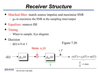
1. Receiver Structure
 Matched filter: match source impulse and maximize SNR
– grx to maximize the SNR at the sampling time/output
 Equalizer: remove ISI
 Timing
– When to sample. Eye diagram
 Decision
– d(i) is 0 or 1 Figure 7.20
Noise na(t)
i ⋅T
d(i) gTx(t) gRx(t) r (iT ) = r0 (iT ) + n(iT )
S
→ max
? N
EE 541/451 Fall 2006

2. Matched Filter
 Input signal s(t)+n(t)
 Maximize the sampled SNR=s(T0)/n(T0) at time T0
EE 541/451 Fall 2006

3. Matched filter example
 Received SNR is maximized at time T0
S
Matched Filter: optimal receive filter for maximized
N
example:
gTx (t ) gTx (−t ) gTx (T0 − t ) = g Rx (t )
T0 t T0 t T0 t
transmit filter receive filter
(matched)
EE 541/451 Fall 2006

4. Equalizer
 When the channel is not ideal, or when signaling is not Nyquist,
There is ISI at the receiver side.
 In time domain, equalizer removes ISR.
 In frequency domain, equalizer flat the overall responses.
 In practice, we equalize the channel response using an equalizer
EE 541/451 Fall 2006

5. Zero-Forcing Equalizer
 The overall response at the detector input must satisfy Nyquist’s
criterion for no ISI:
 The noise variance at the output of the equalizer is:
– If the channel has spectral nulls, there may be significant noise
enhancement.
EE 541/451 Fall 2006

6. Transversal Transversal Zero-Forcing Equalizer
 If Ts<T, we have a fractionally-spaced equalizer
 For no ISI, let:
EE 541/451 Fall 2006

7. Zero-Forcing Equalizer continue
 Zero-forcing equalizer, figure 7.21 and example 7.3
 Example: Consider a baud-rate sampled equalizer for a system
for which
 Design a zero-forcing equalizer having 5 taps.
EE 541/451 Fall 2006

8. MMSE Equalizer
 In the ISI channel model, we need to estimate data input
sequence xk from the output sequence yk
 Minimize the mean square error.
EE 541/451 Fall 2006

9. Adaptive Equalizer
 Adapt to channel changes; training sequence
EE 541/451 Fall 2006

10. Decision Feedback Equalizer
 To use data decisions made on the basis of precursors to take
care of postcursors
 Consists of feedforward, feedback, and decision sections
(nonlinear)
 DFE outperforms the linear equalizer when the channel has
severe amplitude distortion or shape out off.
EE 541/451 Fall 2006

11. Different types of equalizers
 Zero-forcing equalizers ignore the additive noise and may
significantly amplify noise for channels with spectral nulls
 Minimum-mean-square error (MMSE) equalizers minimize the mean-
square error between the output of the equalizer and the transmitted
symbol. They require knowledge of some auto and cross-correlation
functions, which in practice can be estimated by transmitting a known
signal over the channel
 Adaptive equalizers are needed for channels that are time-varying
 Blind equalizers are needed when no preamble/training sequence is
allowed, nonlinear
 Decision-feedback equalizers (DFE’s) use tentative symbol decisions
to eliminate ISI, nonlinear
 Ultimately, the optimum equalizer is a maximum-likelihood sequence
estimator, nonlinear
EE 541/451 Fall 2006

12. Timing Extraction
 Received digital signal needs to be sampled at precise instants.
Otherwise, the SNR reduced. The reason, eye diagram
 Three general methods
– Derivation from a primary or a secondary standard. GPS, atomic
closk
x Tower of base station
x Backbone of Internet
– Transmitting a separate synchronizing signal, (pilot clock, beacon)
x Satellite
– Self-synchronization, where the timing information is extracted
from the received signal itself
x Wireless
x Cable, Fiber
EE 541/451 Fall 2006

13. Example
 Self Clocking, RZ
 Contain some clocking information. PLL
EE 541/451 Fall 2006

14. Timing/Synchronization Block Diagram
 Figure 2.3
 After equalizer, rectifier and clipper
 Timing extractor to get the edge and then amplifier
 Train the phase shifter which is usually PLL
 Limiter gets the square wave of the signal
 Pulse generator gets the impulse responses
EE 541/451 Fall 2006

15. Timing Jitter
 Random forms of jitter: noise, interferences, and mistuning of
the clock circuits.
 Pattern-dependent jitter results from clock mistuning and,
amplitude-to-phase conversion in the clock circuit, and ISI,
which alters the position of the peaks of the input signal
according to the pattern.
 Pattern-dependent jitter propagates
 Jitter reduction
– Anti-jitter circuits
– Jitter buffers
– Dejitterizer
EE 541/451 Fall 2006

16. Bit Error Probability
Noise na(t)
i ⋅T
d(i) gTx(t) gRx(t) r0 (i T ) + n(iT )
We assume: • binary transmission with d (i ) ∈ {d 0 , d1}
• transmission system fulfills 1st Nyquist criterion
• noise n(iT), independent of data source
p N (n )
Probability density function (pdf) of n(iT)
Mean and variance
n
EE 541/451 Fall 2006

17. Conditional pdfs
The transmission system induces two conditional pdfs depending on d (i )
• if d (i ) = d 0 • if d (i ) = d1
p0 ( x ) = p N ( x − d 0 ) p1 ( x) = p N ( x − d1 )
p0 ( x ) p1 ( x)
x
d0 d1 x
EE 541/451 Fall 2006

18. Probability of wrong decisions
Placing a threshold S
p0 ( x ) p1 ( x)
Probability of
wrong decision
x x
d0 S S d1
∞ S
Q0 = ∫ p0 ( x) dx Q1 =
∫ p ( x)dx
1
S −∞
When we define P0 and P1 as equal a-priori probabilities of d 0 and d1
(P0 = P = 1 )
we will get the bit error probability 1 2
∞ S S
Pb = P0Q0 + P Q1 =
1
1
2 ∫s p ( x)dx + ∫ p ( x)dx =
S
0
1
2
−∞
1
1
2 + ∫[
−∞
1
2 p1 ( x) − 1 p0 ( x ) ] dx
2
1 24
4 3
S
1− ∫ p0 ( x ) dx
−∞
EE 541/451 Fall 2006

19. Conditions for illustrative solution
1 d 0 + d1
With  P1 = P0 = and  pN (− x) = pN ( x) ⇒ S=
2
2
S
1 
S
Pb = 1 + ∫ p1 ( x) dx − ∫ p0 ( x ) dx 
2  −∞ −∞ 
d 0 − d1
d +d S ′=
S S= 0 1 S 2
2
∫ p ( x) dx = ∫ p
1 N ( x − d1 )dx ∫ p ( x) dx
1 = ∫p N ( x ′ )d x ′ equivalently
−∞ −∞ −∞ −∞ S
with 
substituting x −d1 = x ′ d −d d −d ∫ p0 ( x ) dx =
d +d
0 1 1 0
2 −∞
for x =S = 0 1 1 2 1
2 = + ∫ p N ( x ′ )d x ′ = − ∫ p N ( x ′ )d x ′ d1 − d 0
d 0 + d1 d 0− d 1 2 0 2 0 1 2
⇒S ′ = − d1= + ∫ p N ( x ' ) dx '
2 2 d −d 1 0 2 0
1 2

Pb = 1 − 2 ∫ p N ( x )dx 
2 0 
EE 541/451 Fall 2006

20. Special Case: Gaussian distributed noise
Motivation: • many independent interferers
• central limit theorem
• Gaussian distribution
d1− d 0
n 2
 x 
2 −
2
−
1 1 2 
e 2σ ∫
2
2σ
pN ( n ) =
2
N
 Pb = 1 − e dx

N
2π σ N 2 2π σ N 0 0

 1 24 
4 3
no closed solution
Definition of Error Function and Error Function Complement
x
2 − x′
2
erf( x) = ∫ e d x′
π 0
erfc( x) = 1 − erf( x )
EE 541/451 Fall 2006

21. Error function and its complement
 function y = Q(x)
y = 0.5*erfc(x/sqrt(2));
2.5
erf(x)
erfc(x)
2
1.5
erf(x), erfc(x)
1
0.5
0
-0.5
-1
-1.5
-3 -2 -1 0 1 2 3
x
EE 541/451 Fall 2006

22. Bit error rate with error function complement
 d1 − d 0
x2 
1 2 1 2 −
 1  d − d0 
∫
2
2σ N
Pb = 1 − e d x  Pb = erfc 1 
2

π 2σ N 0 
2  2 2σ N 
 
Expressions with E S and N 0
antipodal: d1 = + d ; d 0 = − d unipolar d1= + d ; d 0 = 0
1  d −d  1  d  1  d  1  d2 
Pb = erfc  1 0  = erfc   Pb = erfc 
 2 2σ  = erfc 
 2 
2  2 2σ  2  2σ  2  8σ N
2 
 N   N   N   
1  d2  1  SNR  1  d2 / 2  1  SNR 
= erfc   = erfc 
  = erfc   = erfc  
2  2σ N

2  2
  2  2  4σ N  2
2 
 4 
 
d2 ES d2 / 2 ES
SNR = 2 = SNR = 2 =
σN matched N / 2
0 σ N matched N 0 / 2
1  ES  1  ES 
Pb = erfc
 N  Q function Pb = erfc  
2  0  2  2 N0 
 
EE 541/451 Fall 2006

23. Bit error rate for unipolar and antipodal transmission
 BER vs. SNR
theoretical
-1
10 simulation
unipolar
-2
10
BER
antipodal
-3
10
-4
10
-2 0 2 4 6 8 10
ES
in dB
N0
EE 541/451 Fall 2006