communication engineering lab report, 5th sem, electrical engineering, IIT Delhi, eep306

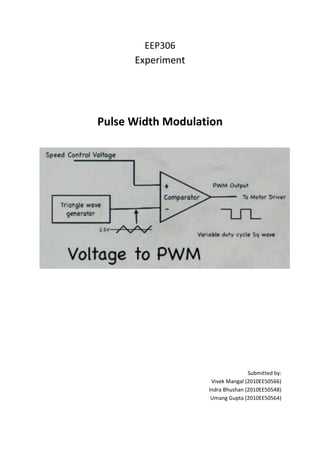
1. EEP306
Experiment
Pulse Width Modulation
Submitted by:
Vivek Mangal (2010EE50566)
Indra Bhushan (2010EE50548)
Umang Gupta (2010EE50564)

2. Introduction:
Pulse width Modulation uses a rectangular pulse wave whose width is modulated resulting in the
variation of the average value of the waveform.
The main advantage of PWM is that power loss in the switching devices is very low. When a switch is
off there is practically no current, and when it is on, there is almost no voltage drop across the
switch. Power loss, being the product of voltage and current, is thus in both cases close to zero.
PWM also works well with digital controls, which, because of their on/off nature, can easily set the
needed duty cycle. PWM has also been used in certain communication systems where its duty cycle
has been used to convey information over a communications channel.
Pulse Position Modulation: The amplitude and width of the pulse generated remains constant,
however the position of pulse appearing in the generated PPM depends on the input. It is often
implemented differentially as differential pulse-position modulation, where each pulse position is
encoded relative to the previous; the receiver only measures the difference in the arrival time of
successive pulses. It has higher noise immunity since all the receiver needs to do is detect the
presence of a pulse at the correct time; the duration and amplitude of the pulse are not important.
Expected PWM outputs can be generated through matlab.
Message signal :

3. Matlab Code for PWM:
%%pwm code
close all
clear all
clc
%%initialisation
f=200;
t=0:0.000025:0.005*2;
fclk=2000;
fs=1/0.000025
fcut=1500;
m=1+0.75*sin(2*pi*f.*t);
saw=1+sawtooth(2*pi*fclk.*t)
o=zeros(1,length(m));
for i=1:length(m)
if m(i)>saw(i)
o(i)=1;
end
end
[b,a]=butter(10,fcut/fs);
mf=filter(b,a,o);
num=b
den=a
bode(tf(num,den))
figure
plot(t,mf,t,m)
title('demodulation, and the original signal')
xlabel('time'); ylabel('amplitude')
figure
plot(t,o)
title('PWM signal')
xlabel('time'); ylabel('amplitude')
figure
plot(t,o,'r',t,m,'black',t,saw,'blue')
title('all signals')
xlabel('time'); ylabel('amplitude')
figure
plot(t,m)
title('msg signal')
xlabel('time'); ylabel('amplitude')

4. PWM signal expected for the given message signal.
The Saw-tooth signal (input in comparator) together with message signal and PWM generated :
Demodulated signal plotted against the message signal :

5. Observation :
Pulse Width Modulation
Input wave shown with its pulse width modulated wave.
1-> Input wave
2 -> Pulse width modulated wave
3 -> Pulse width demodulated wave, observed inverted and lagging in phase with the input wave.

6. Pulse Position Modulation
Input wave shown with its pulse position modulated wave.
1-> Input wave
2 -> Pulse position modulated wave
3 -> Pulse position demodulated wave, observed lagging in phase with the input wave.
Inference :
 The expected output according to matlab is observed experimentally.
 We observe that in PWM, the pulses near the edges of the half cycle are always narrower
than the pulses near the center of the half cycle such that the pulse widths are proportional
to the corresponding amplitude of a sine wave at that portion of the cycle.
 The message input m(t) can be recovered for the PPM signal by passing it through a LPF .