SlideShare une entreprise Scribd logo
1  sur  31
Télécharger pour lire hors ligne
Genetic Algorithms and Evolutionary Computing - Project
Eryk Kulikowski
December 22, 2014
Part I
Implementation
1 Path representation
Additionally to the adjacency representation, already present in the template, path representation
was implemented. The conversion between path and adjacency (and the other way) was also present
in the code. The added functionalities implemented for this project allow for selecting either path or
adjacency representation as default for running the algorithm. This includes:
• Separated run ga methods, one for path, one for adjacency. See also listing 1 (because the
different implementations are redundant, only the path version is included in the appendix).
The run ga implementation also includes an extension for automation of the experiments, see
also section 5.
• Implementation of the fitness function evaluation using the path representation. See listing 2.
• Different versions for executing the mutation (including path improvement) and crossover opera-
tors. This only includes calling transformations of representations where needed, e.g., see listings
3, 11 and 17.
• The GUI was extended to support selecting the representation, see also section 6.
The path representation does not significantly change the quality of the solution or computation
speed. For the computation speed, the fitness evaluation and the crossover operator have greater
influence than conversions between the representations. Also, the fitness evaluation seems to be more
efficient when using adjacency representation (this depends on how Matlab performs matrix operations,
nevertheless, the adjacency fitness evaluation does not require an inner loop in the Matlab code).
Only a small improvement of computation speed can be observed when using path representation in
combination with the crossover operator designed for that representation. Table 1 shows computation
times for path and adjacency representations using the SCX crossover operator and the same parameter
settings for both runs (error percentage is the error compared to the optimal solution for the xqf131
benchmark problem):
Test path adjacency
CPU 370.2132s 378.6447
Error percentage 3.3637 3.9941
Table 1: Difference in computation speed between path and adjacency representations
The percentage error for both examples is within the variation for the chosen operators. More
details on performed experiments can be found in the second part of the report.
1
2 Selection methods
The linear rank selection with Stochastic Universal Sampling was already present in the template,
additionally the following selection methods were implemented and tested (RWS and SUS selection
methods are present in the template making the implementation trivial, see also the code listing for
the corresponding selection methods):
• Roulette Wheel Selection with fitness scaling. The fitness function for TSP is a cost function,
i.e., we are looking for the minimum distance, therefore the fitness scaling takes the highest
distance in the current generation and uses it as minimum (set to 0) and the difference betwee
the shortest and longest distance is the maximum. All values are transformed accordingly. See
also listing 4.
• Stochastic Universal Sampling with fitness scaling. The same fitness scaling as described above,
but in combination with the SUS, see also listing 5.
• K-tournament selection. As this selection method allows setting the selection pressure by the
means of the K-value, this operator was extended in order to support continuous values. If the
K-value is not an integer, then the floored value is taken for the K value and the cut-off value
is then used as a probability for selecting K+1 individuals for the tournament in the particular
selection (i.e., either K or K+1 individuals are selected, with the probability for K+1 equal to
Kvalue − floor(input)). See also listing 6.
• Linear Ranking Roulette Wheel Selection. Roulette Wheel Selection with linear ranking instead
of the fitness scaling. This selection method is similar to the default linear ranking SUS method
provided in the template, except it uses the RWS instead of SUS selection. See also listing 7.
• Non-linear Ranking Roulette Wheel Selection. For the non-linear ranking an exponential func-
tion was used. More in particular, the interval of the exponential function with function values
between 1 and 2 was taken for the ranking, where 1 was subtracted in order to become values
between 0 and 1, i.e., exp(linspace(0, 1.0986, Nind) )−1 was used for ranking of the individuals.
See also listing 8.
• Non-linear Ranking Stochastic Universal Sampling. Non-linear ranking as described above, but
in combination with SUS instead of RWS. See also listing 9.
• O(1) Roulette Wheel Selection. Roulette Wheel selection with fitness scaling as described above,
but implemented according to the paper Roulette-wheel selection via stochastic acceptance by
Adam Lipowski and Dorota Lipowska. See also listing 10.
The O(1) RWS was implemented out of curiosity. Unfortunately, some assumptions about the
distribution of the fitness value among the individuals as described by the authors of the paper do not
hold for the TSP problem. No real performance gain could be measured, mainly due to the fact (as
pointed out during the presentation and discussed in the first section about the representation) that
the most computationally expensive steps are the fitness evaluation and the crossover operator, and
thus the selection method has only limited influence on the total computation time. On the positive
side, this selection method is very easy to implement and it is an interesting approach to the Roulette
Wheel Selection.
The most interesting of the implemented selection methods was the K-tournament as it allows
easily regulating the selection pressure through the choice of the K parameter. Furthermore, the
implemented version allows continuous values for that parameter.
3 Crossover operators
Next to the Alternating Edge Crossover, already present in the template, the following crossover
operators were implemented and tested:
2
Figure 1: Order Crossover (source: Genetic Algorithms and Genetic Programming by M. Affenzeller,
S. Wagner, S. Winkler and A. Beham)
• Order Crossover (OX). This crossover operator is implemented as described in the book Genetic
Algorithms and Genetic Programming by M. Affenzeller, S. Wagner, S. Winkler and A. Beham.
See also figure 1 and listing 12. This operator was implemented because the book described this
operator as one of the better crossover operators for the TSP problem.
• Sequential Constructive Crossover (SCX). This crossover operator is implemented as described in
the paper Genetic Algorithm for the Traveling Salesman Problem using Sequential Constructive
Crossover Operator by Zakir H. Ahmed. This crossover operator is very similar to the Heuristic
Crossover as described in the book Genetic Algorithms and Genetic Programming by M. Affen-
zeller, S. Wagner, S. Winkler and A. Beham. The main difference is that the SCX operates on
path representation and does not randomly resolves cycles, but uses the cities that sequentially
follow the current city in the path, for both parents, and then uses the heuristic (shortest dis-
tance) to chose one city. Therefore, this crossover operator combines the heuristic crossover and
the order crossover in one, very good operator (see also test results in the second part of the
report). See also listing 13.
• Edge Recombination Crossover (ERX). This crossover operator is implemented as described
in the book Genetic Algorithms and Genetic Programming by M. Affenzeller, S. Wagner, S.
Winkler and A. Beham. See also listing 14. This operator was implemented because it is a
popular operator among other students and it is also described in the book as one of the better
operators.
• Heuristic Edge Recombination Crossover (Heuristic ERX). This operator is almost the same
as ERX operator, except that the shortest edge from the edge map is chosen for the offspring,
instead of the edge to the city with the fewest entities in its own edge list (like ERX does) or
prioritizing the edges present in both parents (like Enhanced Edge Recombination Crossover
(EERX) does). See also listing 15. This operator performed very well in the experiments.
The Heuristic ERX and SCX operators came out as best operators from the experiments. See also the
second part of the report for the experiments results.
4 Mutation operators
Next to the Reciprocal Exchange and Simple Inversion mutation operators already present in the
template, the following mutation operators were implemented and tested:
• Insertion (position-based). This operator randomly chooses a city, removes it from the tour and
inserts it at a randomly selected place. See also listing 16.
• Inversion (cut-inversion). This is similar mutation operator to the inversion mutation, but it
reinserts the reversed sub-tour at a random position. See also listing 17.
3
The best operator seems to be the Simple Inversion operator (see the second part of the report
for experiments results) that already was included in the template. This operator changes only two
edges where the selected sub-tour has the same sequence of the visited cities, but in reverse order.
Therefore, this operator introduces new genetic material with a minimal impact on the good tours
and the mutation ratio can be kept high for fast converging operators like SCX and Heuristic ERX.
5 Automation of experiments
For running the experiments, the following elements were implemented:
• Extension of the run ga function to return the relevant results. This function was adapted to
return the used parameters, best result found (distance and the tour), so that they can be written
to file for later analysis when the experiment is finished. See also listing 1.
• Function for running multiple experiments at once in parallel (e.g., experiment8, see also listing
18). This function runs the experiments with different parameters (random or predetermined)
and writes the results in a comma separated values (csv) file for later analysis.
• Work around for the Matlab string concatenation when using parallel computing. String concate-
nation did not work in parallel loop, simple wrapping in a Matlab function solved this problem.
See also listing 19.
• Displaying of the found solution. The graphical visualisation is nod turned on when running
automated experiments (this would be impossible, for example, when running several hundred
experiments at once). Nevertheless, it is interesting to see some solutions found by the algorithm,
a simple function was implemented for that purpose. See also listing 20.
• Automated processing of the data. The resulting csv file as generated by the automated exper-
iments is not easy to process manually. It contains raw data, and for example, the found best
solution is not very useful for statistical analysing the data. Therefore, a Perl script was writ-
ten to process the data (see also listings 21 and 22). More in particular, the script outputs the
following files:
– Transformed csv file in a format usable in other software, like for example R for statistical
analysis.
– File with computed mean distances of the found solutions. For the distances mean compu-
tation, the categorical parameters (crossover, mutation and local improvement operators)
are grouped (the selection method is assumed to be K-tournament with a continuous value
for the K parameter and therefore it is not grouped), and for each unique combination
of these parameters a mean is computed. Also, the best found solution (distance and the
error percentage) are computed, together with the Mean Error Percentage for the given
parameters group. This proved to be very useful for comparing the different operators, etc.
– The means for the CPU time are only applicable when comparing the different selection
methods and are not used in other experiments (the CPU time is not reliable when running
experiments in parallel, but they are reliable when running single experiment on a single
core, this became apparent after running the first set of experiments for selection methods).
See also the second part of this report.
– Best solution found file. This file takes the best solution found from the whole experiment
and outputs the tour, the distance, the error percentage and the used parameters.
– Early convergence file. This file outputs the data where the algorithm was stopped using
the stop percentage, i.e., before reaching the MaxGen number of generations.
The combination of the automated Matlab function with the Perl script for processing the data
proved to be a very efficient way of running the experiments. The tables as shown in the second part
of the report are based on the csv files processed with the Perl script.
4
6 GUI extension
Also the GUI was extended to support all of the implemented parameters. This proved to be useful
for measuring the CPU times (as the algorithm runs on a single core when executed from the GUI).
For example, the results shown in the table 1 in section 1 are generated this way. Figure 2 shows a
screen-shot of the extended GUI (code is not included in the appendix).
Figure 2: Extended GUI
Part II
Experimentation and results
7 Selection methods
These were the first experiments performed. The original idea was to do a kind of grid search for the
best parameters. For the first experiment a minimal set of possible values was chosen (e.g., only two
values: a high value and a low value):
• Comparison of different selection strategies. All implemented selection strategies were going to
be tested, including k-tournament with different k-values (2, 4 and 6). Ten strategies in total.
• High (500) and low (100) value for the number of individuals.
• High (500) and low (100) value for the number of generations.
• High (0.9) and low (0.1) value for the probability of crossover.
• High (0.9) and low (0.1) value for the probability of mutation.
5
• Other parameters were fixed: stop percentage = 0.95, elitist = 0.1, crossover = xalt edges, local
loop = On.
• 5 iteration of each parameter settings group and 3 benchmark problems where used.
• In total: 5 ∗ 3 ∗ 2 ∗ 2 ∗ 2 ∗ 2 ∗ 10 = 2400 experiments.
This approach failed, as the experiments run for a very long time. Running it on multiple machines
would help, but the number of experiments grows exponentially with the size of the grid; i.e., number
of possible values for each parameter, therefore, even on multiple machines the running time would be
very long for a more accurate experiment.
In order to run the first experiment, good values for the parameters were chosen by manual
experimentation (I have already tried different parameters in the exercise session, so I had an idea
what could work with xalt edges operator). More methodical approach is used in later experiments (see
the next section). Finally, the following experiments (among others, only the most relevant experiments
are discussed) were done for the selection strategies:
• Experiment 1 (see also figure 3, the tables in that figure are csv files processed with Perl script
and opened in a spreadsheet processor):
– 10 selection strategies
– 3 problems: Belgian tour (small), benchmark with 380 cities (medium) and benchmark with
711 cities (large)
– 5 runs for each combination of selection strategy/problem
– the parameters: high mutation probability, low crossover probability, 500 generations, 150
individuals
• Experiment 2 (see also figure 4):
– since the first experiment has shown that the selection pressure is the most important factor
for choosing the selection strategy, see also conclusion and interpretations below, different
k values were tested (from low to very high): k = 2, 6, 10, 20, 30, 40, 60
Important conclusions and interpretations:
• K-tournament seems to be a good option. It allows setting the selection pressure with the K-value
and therefore can be easily used with different crossover operators that work better with low or
high selection pressure. Further improvement of allowing continuous values for the K parameter
made it a good choice for experimentation.
• O(1) RWS was not proven. This was more a curiosity, no special attention is given to this
selection method in further experiments.
• Alternating edge crossover does not perform very well. The experiments were more evolutionary
algorithm then genetic algorithm: the selection pressure was set very high (this even resembles
hill climbing algorithm) to obtain good results, crossover rate was low and mutation rate was
high. Better crossover operators were implemented for further testing.
• Good experiment setup is important. With better experiment setup the running time can be
reduced and good parameters can be found more easily. See also the remaining experiments.
The K-tournament selection strategy is used in all remaining experiments. It proved to be very
versatile, allowing turning off the selection pressure (setting the K value to 1), to setting it very high
(large K values lean towards hill climbing algorithms). Further improvements of the K-tournament
are also possible (e.g., adaptive K value for changing the selection pressure during the run of the
algorithm), but it was not investigated. The focus of the remaining experiments was on crossover and
mutation operators.
6
Figure 3: Experiment 1.
Figure 4: Experiment 2.
7
8 Remaining experiments
For the remaining experiments, the problem with 131 cities was used (this was hard enough for all
operators, as globally optimal solutions were not found, and small enough to keep the computation
time limited). It is a benchmark problem with a known optimal solution, so the percentage error was
used to evaluate the experiments. The experiments were also better designed, focusing on the crossover
and mutation operators. The other parameters where kept in a range (determined empirically) that
was big enough so the optimal value was likely included, and small enough to reduce the variation
of the quality of the found solution. The parameter values were chosen at random within that range,
to reduce the influence of these parameter values, allowing a good comparison of the crossover and
mutation operators (the experiment results were consistent, so the statistical techniques as ANOVA or
Regression did not seem to be necessary, it remains a possible improvement to the used methodology).
Many experiments were performed, only the most important of them are discussed:
• Experiment 3 (see also figure 5):
– This experiment compares many different options: 3 crossover operators (SCX, OX and
Alternating Edges), Local Improvement (on or off) and the 4 mutation operators (Insertion,
Reciprocal Exchange, Inversion and Simple Inversion). As it tests different options and it is
intended as a first exploration, the parameter range is large (larger variation of the found
solutions).
– SCX is clearly the winner of this test. The difference between the OX and Alternating Edges
crossovers is less outspoken, with OX performing better than Alternating Edges. Since the
SCX is by a large margin better than the other two, it is chosen for further exploration in
the next experiments.
– Local Improvement does not seem to be important for the SCX operator. It can be explained
by that both, local improvement and SCX are heuristic operators, therefore the Local
Improvement is redundant for the SCX.
• Experiment 4 (see also figure 6):
– This is one of the smaller experiments further exploring the influence of the local improve-
ment, mutation operators and the parameters range for the SCX operator.
– The SCX does not seem to have any advantage in using the local improvement, it even
seems that the SCX works better without it (most likely it is due to the statistical error,
however, there could be small influence by Local Improvement undoing some of the mutation
changes). Since the Local Improvement also requires extra computation, it is turned off in
later experiments.
– The influence of the mutation operators is not clear at this stage. However, the experiments
did allow for further narrowing of the parameter range.
• Experiment 5 (see also figure 7):
– This is a bigger experiment (960 runs of the GA) further exploring the influence of the
mutation operators with a narrower range of the parameters.
– It is clear that the Simple Inversion and Inversion work better than the Insertion and the
Reciprocal Exchange operators. This could be explained by that the first two operators are
less destructive for the tours (and sub-tours), given that the mutation rate is high enough to
introduce new genetic material for the fast converging SCX operator. Best working mutation
rate is around 55%. This is rather high mutation rate, this could be explained by that the
heuristic operator can easily undo many of the mutations, and that the fast convergence
rate of the SCX permits (or even requires) higher mutation rates.
– Parameters that work well: mutation percentage around 55% (as discussed above), crossover
percentage around 70% (this is quite normal rate), population around 300 (more or less
8
twice the number of cities, this is also to be expected), around 5% elite (lower values work
also well, as long as it is not 0%) and low selection pressure with K around 2 (it helps to
preserve genetic diversity for fast convergence operators like SCX). The GA’s were run with
600 generations. However, SCX converges fast and tends to get stuck in a local optimum.
Small improvements can be observed up to 200 generations (they still happen after that, but
at very low rate). Nevertheless, the experiments were run with 600 generations, as sometimes
the algorithm can get ”lucky”, as can be seen for the solution with 1.5% error. This is very
low, more representative values are between 3 and 4 percent, with occasionally the error
percentage dropping below 3% (it drops below 3% more easily for larger populations with
many generations, see also figure 10b, error below 2% remains exceptional).
Figure 5: Experiment 3.
Figure 6: Experiment 4.
Figure 7: Experiment 5.
After running the above described experiments, I wanted to try also other operators, that I could
compare with SCX. I wanted to try the ERX operator, as it was popular among other students, and
9
it was easy to extend it with a heuristic. I have implemented the two operators (ERX and Heuristic
ERX) and run the following experiment:
• Experiment 6 (see also figure 8):
– This is a medium experiment with 480 runs of the GA, the compared operators are the ERX
and Heuristic ERX operators with Simple Inversion and Inversion mutation operators.
– The parameter range is the same as in the experiment 5. This values are also close to
optimal for the Heuristic ERX. However, the ERX works better with much lower mutation
rate (mutation rate around 5% seems to work very well). Nevertheless, even with adapted
mutation rate the error percentage remains higher for the ERX than for Heuristic ERX
(best seen result was around 7%). It could be possible to optimize ERX to obtain even
better results, but it seemed not necessary since it needs many generations (around 600) to
obtain low error percentage, while Heuristic ERX only needs 50 generations to achieve even
lower error rates, while it is also a computationally efficient operator (see the test below).
– Heuristic ERX is a very good operator. The results suggest that is even better than SCX.
Even if this is due to a statistical error, the ERX is computationally more efficient than
SCX, making it the first choice. From the obtained results: Heuristic ERX is best, followed
by SCX, ERX, OX and Alternating edges at the end.
– The Simple Inversion operator was again the best from the tests, making it the best muta-
tion operator among the tested operators.
Figure 8: Experiment 6.
In order to compare the computational times for the different crossover operators, a test was
run where the parameters where kept the same for all operators, running for 200 generations and
population of 300. The results are shown in table 2. From that table, it is noticeable that the ERX is
a relatively fast operator, as it has an opinion of being expensive due to the need of the construction
of the edge map. It is almost as fast as OX. Even the Heuristic ERX is very fast, with only a very
small difference compared to the ERX. It is clear that SCX is very expensive. This numbers could
be different for other programming environments than Matlab or different implementation choices.
HERX is clearly the best operator that I have implemented.
Test AltEdges OX SCX ERX HERX
CPU 110.1591s 26.8284 170.0268s 29.3589 30.2929
Error percentage 269.7051 165.3390 6.4763 133.4527 3.9726
Table 2: Difference in computation speed between the implemented crossover operators.
Figure 9 shows the best solutions as found by the SCX and HERX operators during the above
described experiments (experiment 5 and 6) compared to the optimal solution for the xqf131 bench-
mark problems. Figure 10 shows the results of a single-run experiments with the HERX operator for
the different benchmark problems (belgiumtour, xqf131, bcl380 and rbx711).
10
(a) SCX (1.52% error) (b) HERX (1.62% error)
(c) Optimal solution
Figure 9: Comparison of the solutions found in the experiments with the optimal solution.
(a) belgiumtour (b) xqf131 (2.28% error)
(c) bcl380 (3.97% error) (d) rbx711 (3.59% error)
Figure 10: Single-run experiments for the bechmark problems.
11
Part III
Appendix: Code
Listings
1 code/run ga path.m . . . . . . . . . . . . . . . . . . . . . . . . . . . . . . . . . . . . . 12
2 code/tspfun path.m . . . . . . . . . . . . . . . . . . . . . . . . . . . . . . . . . . . . . 14
3 code/tsp ImprovePopulation path.m . . . . . . . . . . . . . . . . . . . . . . . . . . . . 14
4 code/fitsc rws.m . . . . . . . . . . . . . . . . . . . . . . . . . . . . . . . . . . . . . . . 15
5 code/fitsc sus.m . . . . . . . . . . . . . . . . . . . . . . . . . . . . . . . . . . . . . . . . 15
6 code/k tournament.m . . . . . . . . . . . . . . . . . . . . . . . . . . . . . . . . . . . . 16
7 code/lin rank rws.m . . . . . . . . . . . . . . . . . . . . . . . . . . . . . . . . . . . . . 16
8 code/non lin rank rws.m . . . . . . . . . . . . . . . . . . . . . . . . . . . . . . . . . . . 17
9 code/non lin rank sus.m . . . . . . . . . . . . . . . . . . . . . . . . . . . . . . . . . . . 17
10 code/o1 rws.m . . . . . . . . . . . . . . . . . . . . . . . . . . . . . . . . . . . . . . . . 18
11 code/erx.m . . . . . . . . . . . . . . . . . . . . . . . . . . . . . . . . . . . . . . . . . . 19
12 code/cross ox.m . . . . . . . . . . . . . . . . . . . . . . . . . . . . . . . . . . . . . . . . 20
13 code/cross scx.m . . . . . . . . . . . . . . . . . . . . . . . . . . . . . . . . . . . . . . . 21
14 code/cross erx.m . . . . . . . . . . . . . . . . . . . . . . . . . . . . . . . . . . . . . . . 22
15 code/cross herx.m . . . . . . . . . . . . . . . . . . . . . . . . . . . . . . . . . . . . . . 23
16 code/insertion.m . . . . . . . . . . . . . . . . . . . . . . . . . . . . . . . . . . . . . . . 25
17 code/inversion.m . . . . . . . . . . . . . . . . . . . . . . . . . . . . . . . . . . . . . . . 25
18 code/experiment8.m . . . . . . . . . . . . . . . . . . . . . . . . . . . . . . . . . . . . . 26
19 code/add strings.m . . . . . . . . . . . . . . . . . . . . . . . . . . . . . . . . . . . . . . 28
20 code/disp sol.m . . . . . . . . . . . . . . . . . . . . . . . . . . . . . . . . . . . . . . . . 28
21 code/run.pl . . . . . . . . . . . . . . . . . . . . . . . . . . . . . . . . . . . . . . . . . . 28
22 code/transform.pl . . . . . . . . . . . . . . . . . . . . . . . . . . . . . . . . . . . . . . . 28
Listing 1: code/run ga path.m
function r e s u l t = run ga path (x , y , NIND, MAXGEN, NVAR, ELITIST , STOP PERCENTAGE,
PR CROSS, PR MUT, CROSSOVER, LOCALLOOP, ah1 , ah2 , ah3 , SELECTION, KVALUE, MUTATION)
% usage : run ga path (x , y ,
% NIND, MAXGEN, NVAR,
% ELITIST , STOP PERCENTAGE,
% PR CROSS, PR MUT, CROSSOVER,
% ah1 , ah2 , ah3 )
%
%
% x , y : coordinates of the c i t i e s
% NIND: number of i n d i v i d u a l s
% MAXGEN: maximal number of generations
% ELITIST : percentage of e l i t e population
% STOP PERCENTAGE: percentage of equal f i t n e s s ( stop criterium )
% PR CROSS: p r o b a b i l i t y f o r crossover
% PR MUT: p r o b a b i l i t y f o r mutation
% CROSSOVER: the crossover operator
% c a l c u l a t e distance matrix between each pair of c i t i e s
% ah1 , ah2 , ah3 : axes handles to v i s u a l i s e tsp
% edited 16/11/2014 by Eryk Kulikowski : added return to the function f o r running
experiments whithout gui
% and changed the d ef a ul t representation to path representation
{NIND MAXGEN NVAR ELITIST STOP PERCENTAGE PR CROSS PR MUT CROSSOVER LOCALLOOP SELECTION
KVALUE ’ path ’ MUTATION}
GGAP = 1 − ELITIST ;
mean fits=zeros (1 ,MAXGEN+1) ;
worst=zeros (1 ,MAXGEN+1) ;
12
Dist=zeros (NVAR,NVAR) ;
f o r i =1: s i z e (x , 1 )
f o r j =1: s i z e (y , 1 )
Dist ( i , j )=sqrt (( x( i )−x( j ) ) ˆ2+(y( i )−y( j ) ) ˆ2) ;
end
end
% i n i t i a l i z e population
Chrom=zeros (NIND,NVAR) ;
f o r row=1:NIND
% PATH %
%Chrom(row , : )=path2adj ( randperm (NVAR) ) ;
Chrom(row , : )=randperm (NVAR) ;
end
gen=0;
% number of i n d i v i d u a l s of equal f i t n e s s needed to stop
stopN=c e i l (STOP PERCENTAGE∗NIND) ;
% evaluate i n i t i a l population
% PATH %
%ObjV = tspfun (Chrom , Dist ) ;
ObjV = tspfun path (Chrom , Dist ) ;
best=zeros (1 ,MAXGEN) ;
% generational loop
while gen<MAXGEN
sObjV=sort (ObjV) ;
best ( gen+1)=min(ObjV) ;
minimum=best ( gen+1) ;
mean fits ( gen+1)=mean(ObjV) ;
worst ( gen+1)=max(ObjV) ;
f o r t =1: s i z e (ObjV , 1 )
i f (ObjV( t )==minimum)
break ;
end
end
best found = Chrom( t , : ) ;
% PATH %
%visualizeTSP (x , y , adj2path (Chrom( t , : ) ) , minimum , ah1 , gen , best , mean fits ,
worst , ah2 , ObjV , NIND, ah3 ) ;
visualizeTSP (x , y , Chrom( t , : ) , minimum , ah1 , gen , best , mean fits , worst , ah2
, ObjV , NIND, ah3 ) ;
i f (sObjV( stopN )−sObjV (1) <= 1e −15)
break ;
end
%assign f i t n e s s values to e n t i r e population
%FitnV=ranking (ObjV) ;
%s e l e c t i n d i v i d u a l s f o r breeding
%SelCh=s e l e c t ( ’ sus ’ , Chrom , FitnV , GGAP) ;
SelCh=f e v a l (SELECTION, Chrom , ObjV , GGAP, KVALUE) ;
%recombine i n d i v i d u a l s ( crossover )
% PATH %
%SelCh = recombin (CROSSOVER, SelCh ,PR CROSS, Dist ) ;
PATH CROSSOVER = add strings (CROSSOVER, ’ path ’ ) ;
SelCh = recombin (PATH CROSSOVER, SelCh ,PR CROSS, Dist ) ;
% PATH % − see mutateTSP
%SelCh=mutateTSP ( ’ inversion ’ , SelCh ,PR MUT) ;
SelCh=mutateTSP path (MUTATION, SelCh ,PR MUT) ;
%evaluate o f f s pr i n g , c a l l o b j e c t i v e function
% PATH %
%ObjVSel = tspfun ( SelCh , Dist ) ;
ObjVSel = tspfun path ( SelCh , Dist ) ;
%r e i n s e r t o f f s p r i n g into population
[ Chrom ObjV]= r e i n s (Chrom , SelCh ,1 ,1 , ObjV , ObjVSel ) ;
% PATH % − see tsp ImprovePopulation
%Chrom = tsp ImprovePopulation (NIND, NVAR, Chrom ,LOCALLOOP, Dist ) ;
Chrom = tsp ImprovePopulation path (NIND, NVAR, Chrom ,LOCALLOOP, Dist ) ;
%increment generation counter
13
gen=gen+1;
end
r e s u l t = {NIND MAXGEN NVAR ELITIST STOP PERCENTAGE PR CROSS PR MUT CROSSOVER
LOCALLOOP SELECTION KVALUE gen minimum ’ path ’ MUTATION best found };
end
Listing 2: code/tspfun path.m
% tspfun path .m
% ObjVal = tspfun path (Phen , Dist )
% Implementation of the TSP f i t n e s s function
% Phen contains the phenocode of the matrix coded in path representation
% Dist i s the matrix with precalculated distances between each pair of c i t i e s
% ObjVal i s a vector with the f i t n e s s values f o r each candidate tour (=each row of Phen
)
%
% Author : Eryk Kulikowski
% Date : 20−Nov−2014
function ObjVal = tspfun path (Phen , Dist ) ;
ObjVal = zeros ( s i z e (Phen , 1 ) ,1) ;
f o r k=1: s i z e (Phen , 1 )
ObjVal (k)=Dist (Phen(k , 1 ) ,Phen(k , s i z e (Phen , 2 ) ) ) ;
f o r t = 1: s i z e (Phen , 2 )−1
ObjVal (k)=ObjVal (k)+Dist (Phen(k , t ) ,Phen(k , t+1)) ;
end
end
end
% End of function
Listing 3: code/tsp ImprovePopulation path.m
% tsp ImprovePopulation path .m
% Author : Mike Matton
%
% This function improves a tsp population by removing l o c a l loops from
% each i n d i v i d u a l .
%
% Syntax : improvedPopulation = tsp ImprovePopulation path ( popsize , n c i t i e s , pop ,
improve , d i s t s )
%
% Input parameters :
% popsize − The population s i z e
% n c i t i e s − the number of c i t i e s
% pop − the current population ( adjacency representation )
% improve − Improve the population (0 = no improvement , <>0 = improvement )
% d i s t s − distance matrix with distances between the c i t i e s
%
% Output parameter :
% improvedPopulation − the new population a f t e r loop removal ( i f improve
% <> 0 , e l s e the unchanged population ) .
function newpop = tsp ImprovePopulation path ( popsize , n c i t i e s , pop , improve , d i s t s )
i f ( improve )
f o r i =1: popsize
% PATH %
%r e s u l t = improve path ( n c i t i e s , adj2path ( pop ( i , : ) ) , d i s t s ) ;
r e s u l t = improve path ( n c i t i e s , pop ( i , : ) , d i s t s ) ;
% PATH %
%pop ( i , : ) = path2adj ( r e s u l t ) ;
14
end
end
newpop = pop ;
Listing 4: code/fitsc rws.m
% FITSC RWS.M ( FITness SCaling Roulette Wheel S e l e c t i o n )
%
% This function performs Roulette Wheel S e l e c t i o n with f i t n e s s s c a l i n g .
%
% Syntax : SelCh = f i t s c r w s (Chrom , ObjV , GGAP, KValue )
%
% Input parameters :
% Chrom − Matrix containing the i n d i v i d u a l s ( parents ) of the current
% population . Each row corresponds to one i n d i v i d u a l .
% ObjV − Column vector containing the o b j e c t i v e values of the
% i n d i v i d u a l s in the current population ( cost values ) .
% GGAP − Rate of i n d i v i d u a l s to be s e l e c t e d
% i f omitted 1.0 i s assumed
% KValue − ( optional ) only a pp li ca bl e f o r k−tournament s e l e c t i o n ( ignore )
%
% Output parameters :
% SelCh − Matrix containing the s e l e c t e d i n d i v i d u a l s .
% Author : Eryk Kulikowski
% Date : 16−Nov−2014
function SelCh = f i t s c r w s (Chrom , ObjV , GGAP, KValue )
% Assign f i t n e s s values to e n t i r e population
Omax = max( ObjV ) ;
FitnV = Omax − ObjV ;
%FitnV = exp (Omax − ObjV) −1.0;
% S e l e c t i n d i v i d u a l s f o r breeding
SelCh=s e l e c t ( ’ rws ’ , Chrom , FitnV , GGAP) ;
end
% End of function
Listing 5: code/fitsc sus.m
% FITSC SUS .M ( FITness SCaling Stochastic Universal Sampling )
%
% This function performs Stochastic Universal Sampling with f i t n e s s s c a l i n g .
%
% Syntax : SelCh = f i t s c s u s (Chrom , ObjV , GGAP, KValue )
%
% Input parameters :
% Chrom − Matrix containing the i n d i v i d u a l s ( parents ) of the current
% population . Each row corresponds to one i n d i v i d u a l .
% ObjV − Column vector containing the o b j e c t i v e values of the
% i n d i v i d u a l s in the current population ( cost values ) .
% GGAP − Rate of i n d i v i d u a l s to be s e l e c t e d
% i f omitted 1.0 i s assumed
% KValue − ( optional ) only a pp li ca bl e f o r k−tournament s e l e c t i o n ( ignore )
%
% Output parameters :
% SelCh − Matrix containing the s e l e c t e d i n d i v i d u a l s .
% Author : Eryk Kulikowski
% Date : 16−Nov−2014
function SelCh = f i t s c s u s (Chrom , ObjV , GGAP, KValue )
15
% Assign f i t n e s s values to e n t i r e population
Omax = max( ObjV ) ;
FitnV = Omax − ObjV ;
%FitnV = exp (Omax − ObjV) −1.0;
% S e l e c t i n d i v i d u a l s f o r breeding
SelCh=s e l e c t ( ’ sus ’ , Chrom , FitnV , GGAP) ;
end
% End of function
Listing 6: code/k tournament.m
% KTOURNAMENT.M (K−TOURNAMENT s e l e c t i o n )
%
% This function performs k tournament s e l e c t i o n .
%
% Syntax : SelCh = k tournament (Chrom , ObjV , GGAP, KValue )
%
% Input parameters :
% Chrom − Matrix containing the i n d i v i d u a l s ( parents ) of the current
% population . Each row corresponds to one i n d i v i d u a l .
% ObjV − Column vector containing the o b j e c t i v e values of the
% i n d i v i d u a l s in the current population ( cost values ) .
% GGAP − Rate of i n d i v i d u a l s to be s e l e c t e d i f omitted 1.0 i s assumed
% KValue − Number of i n d i v i d u a l s p a r t i c i p a t i n g in a tournament
% ( r e g u l a t e s s e l e c t i o n pressure )
%
% Output parameters :
% SelCh − Matrix containing the s e l e c t e d i n d i v i d u a l s .
% Author : Eryk Kulikowski
% Date : 15−Nov−2014
function SelCh = k tournament (Chrom , ObjV , GGAP, KValue )
% Compute number of new i n d i v i d u a l s ( to s e l e c t )
[ Nind , ans ] = s i z e ( ObjV ) ;
NSel=max( f l o o r ( Nind∗GGAP+.5) ,2) ;
% S e l e c t i n d i v i d u a l s f o r breeding
SelCh = [ ] ;
f o r i =1:NSel
RowIndex = randi ( Nind ) ;
K = f l o o r ( KValue ) ;
pK = KValue − K;
i f rand<pK
K = K+1;
end
f o r j =1:(K − 1)
RowIndex2 = randi ( Nind ) ;
i f ObjV( RowIndex ) > ObjV( RowIndex2 ) ;
RowIndex = RowIndex2 ;
end
end
SelCh = [ SelCh ; Chrom(RowIndex , : ) ] ;
end
end
% End of function
Listing 7: code/lin rank rws.m
% LIN RANK RWS.M ( LINear RANK RWS s e l e c t i o n )
%
% This function performs Roulette Wheel S e l e c t i o n with l i n e a r ranking .
%
% Syntax : SelCh = lin rank rws (Chrom , ObjV , GGAP, KValue )
%
16
% Input parameters :
% Chrom − Matrix containing the i n d i v i d u a l s ( parents ) of the current
% population . Each row corresponds to one i n d i v i d u a l .
% ObjV − Column vector containing the o b j e c t i v e values of the
% i n d i v i d u a l s in the current population ( cost values ) .
% GGAP − Rate of i n d i v i d u a l s to be s e l e c t e d
% i f omitted 1.0 i s assumed
% KValue − ( optional ) only a pp li ca bl e f o r k−tournament s e l e c t i o n ( ignore )
%
% Output parameters :
% SelCh − Matrix containing the s e l e c t e d i n d i v i d u a l s .
% Author : Eryk Kulikowski
% Date : 16−Nov−2014
function SelCh = lin rank rws (Chrom , ObjV , GGAP, KValue )
% Assign f i t n e s s values to e n t i r e population
FitnV=ranking (ObjV) ;
% S e l e c t i n d i v i d u a l s f o r breeding
SelCh=s e l e c t ( ’ rws ’ , Chrom , FitnV , GGAP) ;
end
% End of function
Listing 8: code/non lin rank rws.m
% NON LIN RANK RWS.M (NON LINear RANK RWS s e l e c t i o n )
%
% This function performs Roulette Wheel S e l e c t i o n with non l i n e a r ranking .
%
% Syntax : SelCh = non lin rank rws (Chrom , ObjV , GGAP, KValue )
%
% Input parameters :
% Chrom − Matrix containing the i n d i v i d u a l s ( parents ) of the current
% population . Each row corresponds to one i n d i v i d u a l .
% ObjV − Column vector containing the o b j e c t i v e values of the
% i n d i v i d u a l s in the current population ( cost values ) .
% GGAP − Rate of i n d i v i d u a l s to be s e l e c t e d
% i f omitted 1.0 i s assumed
% KValue − ( optional ) only a pp li ca bl e f o r k−tournament s e l e c t i o n ( ignore )
%
% Output parameters :
% SelCh − Matrix containing the s e l e c t e d i n d i v i d u a l s .
% Author : Eryk Kulikowski
% Date : 16−Nov−2014
function SelCh = non lin rank rws (Chrom , ObjV , GGAP, KValue )
% Assign f i t n e s s values to e n t i r e population
%RFun = [ 2 . 0 1 ] ;
[ Nind , ans ] = s i z e ( ObjV ) ;
RFun = exp ( l i n s p a c e (0 ,1.0986 , Nind ) ’) −1;
FitnV=ranking (ObjV , RFun) ;
% S e l e c t i n d i v i d u a l s f o r breeding
SelCh=s e l e c t ( ’ rws ’ , Chrom , FitnV , GGAP) ;
end
% End of function
Listing 9: code/non lin rank sus.m
% NON LIN RANK SUS.M (NON LINear RANK SUS s e l e c t i o n )
%
% This function performs Stochastic Universal Sampling with non l i n e a r ranking .
17
%
% Syntax : SelCh = non lin rank sus (Chrom , ObjV , GGAP, KValue )
%
% Input parameters :
% Chrom − Matrix containing the i n d i v i d u a l s ( parents ) of the current
% population . Each row corresponds to one i n d i v i d u a l .
% ObjV − Column vector containing the o b j e c t i v e values of the
% i n d i v i d u a l s in the current population ( cost values ) .
% GGAP − Rate of i n d i v i d u a l s to be s e l e c t e d
% i f omitted 1.0 i s assumed
% KValue − ( optional ) only a pp li ca bl e f o r k−tournament s e l e c t i o n ( ignore )
%
% Output parameters :
% SelCh − Matrix containing the s e l e c t e d i n d i v i d u a l s .
% Author : Eryk Kulikowski
% Date : 16−Nov−2014
function SelCh = non lin rank sus (Chrom , ObjV , GGAP, KValue )
% Assign f i t n e s s values to e n t i r e population
%RFun = [ 2 . 0 1 ] ;
[ Nind , ans ] = s i z e ( ObjV ) ;
RFun = exp ( l i n s p a c e (0 ,1.0986 , Nind ) ’) −1;
FitnV=ranking (ObjV , RFun) ;
% S e l e c t i n d i v i d u a l s f o r breeding
SelCh=s e l e c t ( ’ sus ’ , Chrom , FitnV , GGAP) ;
end
% End of function
Listing 10: code/o1 rws.m
% O1 RWS.M (O(1) r o u l e t t e wheel s e l e c t i o n )
%
% This function performs O(1) ( constant time ) r o u l e t t e wheel s e l e c t i o n .
% Based on ” Roulette−wheel s e l e c t i o n via s t o c h a s t i c acceptance ” paper
% by Adam Lipowski and Dorota Lipowska .
%
% Syntax : SelCh = o1 rws (Chrom , ObjV , GGAP, KValue )
%
% Input parameters :
% Chrom − Matrix containing the i n d i v i d u a l s ( parents ) of the current
% population . Each row corresponds to one i n d i v i d u a l .
% ObjV − Column vector containing the o b j e c t i v e values of the
% i n d i v i d u a l s in the current population ( cost values ) .
% GGAP − Rate of i n d i v i d u a l s to be s e l e c t e d
% i f omitted 1.0 i s assumed
% KValue − ( optional ) only a pp li ca bl e f o r k−tournament s e l e c t i o n ( ignore )
%
% Output parameters :
% SelCh − Matrix containing the s e l e c t e d i n d i v i d u a l s .
% Author : Eryk Kulikowski
% Date : 15−Nov−2014
function SelCh = o1 rws (Chrom , ObjV , GGAP, KValue )
% Compute number of new i n d i v i d u a l s ( to s e l e c t )
[ Nind , ans ] = s i z e ( ObjV ) ;
NSel=max( f l o o r ( Nind∗GGAP+.5) ,2) ;
% Assign f i t n e s s values to e n t i r e population
Omax = max( ObjV ) ;
FitnV = Omax − ObjV ;
%FitnV = exp (Omax − ObjV) −1.0;
% S e l e c t i n d i v i d u a l s f o r breeding
18
SelCh = [ ] ;
Wmax = max( FitnV ) ;
f o r i =1:NSel
RowIndex = NaN;
IndSelected = f a l s e ;
while not ( IndSelected )
RowIndex = randi ( Nind ) ;
pSelect = FitnV ( RowIndex ) /Wmax;
i f pSelect > rand (1)
IndSelected = true ;
end
end
SelCh = [ SelCh ; Chrom(RowIndex , : ) ] ;
end
end
% End of function
Listing 11: code/erx.m
% ERX.M ( Edge Recombination Crossover )
%
% Edge Recombination Crossover as described in the book ” Genetic Algorithms and Genetic
Programming” by
% M. A f f e n z e l l e r , S . Wagner , S . Winkler and A. Beham .
%
% Syntax : NewChrom = erx (OldChrom , XOVR, Dist )
%
% Input parameters :
% OldChrom − Matrix containing the chromosomes of the old
% population . Each l i n e corresponds to one i n d i v i d u a l
% ( in any form , not n e c e s s a r i l y r e a l values ) .
% XOVR − Probability of recombination occurring between p a i r s
% of i n d i v i d u a l s .
% Dist − the matrix with precalculated distances between each pair of c i t i e s
%
% Output parameter :
% NewChrom − Matrix containing the chromosomes of the population
% a f t e r mating , ready to be mutated and/ or evaluated ,
% in the same format as OldChrom .
% Author : Eryk Kulikowski
% Date : 13−Dec−2014
function NewChrom = erx (OldChrom , XOVR, Dist )
i f nargin < 2 , XOVR = NaN; end
[ rows , c o l s ]= s i z e (OldChrom) ;
maxrows=rows ;
i f rem( rows , 2 ) ˜=0
maxrows=maxrows−1;
end
f o r row =1:2: maxrows
% crossover of the two chromosomes
% r e s u l t s in 2 o f f s p r i n g s
i f rand<XOVR % recombine with a given p r o b a b i l i t y
% PATH %
%NewChrom(row , : ) =c r o s s e r x ( [ OldChrom(row , : ) ; OldChrom( row +1 ,:) ] ) ;
%NewChrom( row +1 ,:)=c r o s s e r x ( [ OldChrom( row +1 ,:) ; OldChrom(row , : ) ] ) ;
NewChrom(row , : )=path2adj ( c r o s s e r x ( [ adj2path (OldChrom(row , : ) ) ; adj2path (OldChrom( row
+1 ,:) ) ] ) ) ;
NewChrom( row +1 ,:)=path2adj ( c r o s s e r x ( [ adj2path (OldChrom( row +1 ,:) ) ; adj2path (OldChrom
(row , : ) ) ] ) ) ;
19
e l s e
NewChrom(row , : )=OldChrom(row , : ) ;
NewChrom( row +1 ,:)=OldChrom( row +1 ,:) ;
end
end
i f rem( rows , 2 ) ˜=0
NewChrom( rows , : )=OldChrom( rows , : ) ;
end
end
% End of function
Listing 12: code/cross ox.m
% CROSS OX.M (CROSSover operator : Order Crossover )
%
% Low l e v e l function to perform recombination of two parrents into one o f f s p r i n g using
the
% Order Crossover as described in the book ” Genetic Algorithms and Genetic Programming”
by
% M. A f f e n z e l l e r , S . Wagner , S . Winkler and A. Beham
%
% Syntax : Offspring = cross ox ( Parents )
%
% Input parameters :
% Parents − Matrix containing the 2 i n d i v i d u a l s ( parents as rows ) to be recombined
.
% This operator assumes ”path” representation .
% Dist − the matrix with precalculated distances between each pair of c i t i e s
%
% Output parameters :
% Offspring − One row containing the constructed o f f s p r i n g i n d i v i d u a l .
% Author : Eryk Kulikowski
% Date : 21−Nov−2014
function Offspring = cross ox ( Parents , Dist ) ;
c o l s = s i z e ( Parents , 2 ) ;
Offspring = zeros (1 , c o l s ) ;
parent1 = Parents ( 1 , : ) ;
parent2 = Parents ( 2 , : ) ;
% choose a subtour in the f i r s t parrent and copy i t to the o f f s p r i n g
rndi=zeros (1 ,2) ;
while rndi (1)==rndi (2)
rndi=rand int ( 1 , 2 , [ 1 c o l s ] ) ;
end
rndi = sort ( rndi ) ;
Offspring ( rndi (1) : rndi (2) ) = parent1 ( rndi (1) : rndi (2) ) ;
% cancel the c i t i e s present in the subtour from the second parent
f o r i=rndi (1) : rndi (2)
index = find ( parent2 == Offspring ( i ) ) ;
parent2 ( index ) = 0;
end
% i n s e r t the remaining c i t i e s from parent two into the o f f s p r i n g
node = 1;
f o r i =1: rndi (1)−1
while parent2 ( node )==0
node = node +1;
end
Offspring ( i ) = parent2 ( node ) ;
node = node +1;
end
f o r i=rndi (2) +1: c o l s
while parent2 ( node )==0
node = node +1;
20
end
Offspring ( i ) = parent2 ( node ) ;
node = node +1;
end
end
% end function
Listing 13: code/cross scx.m
% CROSS SCX.M (CROSSover operator : Sequential Constructive Crossover )
%
% Low l e v e l function to perform recombination of two parrents into one o f f s p r i n g using
the Sequential
% Constructive Crossover as described in the paper ” Genetic Algorithm f o r the Traveling
Salesman
% Problem using Sequential Constructive Crossover Operator” by Zakir H. Ahmed.
%
% Syntax : Offspring = c r o s s s c x ( Parents , Dist )
%
% Input parameters :
% Parents − Matrix containing the 2 i n d i v i d u a l s ( parents as rows ) to be recombined
.
% This operator assumes ”path” representation .
% Dist − the matrix with precalculated distances between each pair of c i t i e s
%
% Output parameters :
% Offspring − One row containing the constructed o f f s p r i n g i n d i v i d u a l .
% Author : Eryk Kulikowski
% Date : 20−Nov−2014
function Offspring = c r o s s s c x ( Parents , Dist ) ;
c o l s = s i z e ( Parents , 2 ) ;
Offspring = zeros (1 , c o l s ) ;
parent1 = Parents ( 1 , : ) ;
parent2 = Parents ( 2 , : ) ;
% node ” s t a r t i n d e x ” from parent one i s the f i r s t l e g i t i m a t e node that goes into
o f s s p r i n g
s t a r t i n d e x=rand int ( 1 , 1 , [ 1 c o l s ] ) ;
offspringNode = parent1 ( s t a r t i n d e x ) ;
Offspring (1) = offspringNode ;
pcn1 = s t a r t i n d e x ;
pcn2 = find ( parent2 == offspringNode ) ;
f o r node = 2: c o l s
% find the l e g i t i m a t e node f o r parrent 1
parent1 ( pcn1 ) = 0;
parent2 ( pcn2 ) = 0;
lnp1 = 0;
while (( lnp1 == 0) & ( pcn1 < c o l s ) )
pcn1 = pcn1 + 1;
lnp1 = parent1 ( pcn1 ) ;
end
i f ( lnp1 == 0)
% s t a r t from the beginning of the chromosome
pcn1 = 0;
while ( lnp1 == 0)
pcn1 = pcn1 + 1;
lnp1 = parent1 ( pcn1 ) ;
end
end
% the same f o r parrent two
lnp2 = 0;
while (( lnp2 == 0) & ( pcn2 < c o l s ) )
pcn2 = pcn2 + 1;
lnp2 = parent2 ( pcn2 ) ;
end
21
i f ( lnp2 == 0)
% s t a r t from the beginning of the chromosome
pcn2 = 0;
while ( lnp2 == 0)
pcn2 = pcn2 + 1;
lnp2 = parent2 ( pcn2 ) ;
end
end
% choose the l g i t i m a t e node ( lnp1 or lnp2 ) with the lower distance
d1 = Dist ( offspringNode , lnp1 ) ;
d2 = Dist ( offspringNode , lnp2 ) ;
chosenNode = lnp2 ;
i f ( d2 < d1 )
chosenNode = lnp2 ;
pcn1 = find ( parent1 == chosenNode ) ;
e l s e
chosenNode = lnp1 ;
pcn2 = find ( parent2 == chosenNode ) ;
end
offspringNode = chosenNode ;
Offspring ( node ) = offspringNode ;
end
end
% end function
Listing 14: code/cross erx.m
% CROSS ERX.M (CROSSover operator : Edge Recombination Crossover )
%
% Low l e v e l function to perform recombination of two parrents into one o f f s p r i n g using
the Edge
% Recombination Crossover as described in the book ” Genetic Algorithms and Genetic
Programming” by
% M. A f f e n z e l l e r , S . Wagner , S . Winkler and A. Beham
%
% Syntax : Offspring = c r o s s e r x ( Parents )
%
% Input parameters :
% Parents − Matrix containing the 2 i n d i v i d u a l s ( parents as rows ) to be recombined
.
% This operator assumes ”path” representation .
%
% Output parameters :
% Offspring − One row containing the constructed o f f s p r i n g i n d i v i d u a l .
% Author : Eryk Kulikowski
% Date : 13−12−2014
function Offspring = c r o s s e r x ( Parents ) ;
c o l s = s i z e ( Parents , 2 ) ;
Offspring = zeros (1 , c o l s ) ;
edgeMap = zeros (5 , c o l s ) ;
f o r i = 1:2
i f (( edgeMap (1 , Parents ( i , 1 ) ) <2) | | (( edgeMap (2 , Parents ( i , 1 ) )˜=Parents ( i , c o l s ) ) && (
edgeMap (3 , Parents ( i , 1 ) )˜=Parents ( i , c o l s ) ) && (edgeMap (4 , Parents ( i , 1 ) )˜=Parents ( i ,
c o l s ) ) ) )
edgeMap (1 , Parents ( i , 1 ) ) = edgeMap (1 , Parents ( i , 1 ) ) + 1;
edgeMap(edgeMap (1 , Parents ( i , 1 ) ) +1, Parents ( i , 1 ) ) = Parents ( i , c o l s ) ;
end
i f (( edgeMap (1 , Parents ( i , c o l s ) ) <2) | | (( edgeMap (2 , Parents ( i , c o l s ) )˜=Parents ( i , 1 ) )
&& (edgeMap (3 , Parents ( i , c o l s ) )˜=Parents ( i , 1 ) ) && (edgeMap (4 , Parents ( i , c o l s ) )˜=
Parents ( i , 1 ) ) ) )
edgeMap (1 , Parents ( i , c o l s ) ) = edgeMap (1 , Parents ( i , c o l s ) ) + 1;
edgeMap(edgeMap (1 , Parents ( i , c o l s ) ) +1, Parents ( i , c o l s ) ) = Parents ( i , 1 ) ;
end
f o r j =1:( cols −1)
22
i f (( edgeMap (1 , Parents ( i , j ) ) <2) | | (( edgeMap (2 , Parents ( i , j ) )˜=Parents ( i , j +1)) &&
(edgeMap (3 , Parents ( i , j ) )˜=Parents ( i , j +1)) && (edgeMap (4 , Parents ( i , j ) )˜=Parents ( i , j
+1)) ) )
edgeMap (1 , Parents ( i , j ) ) = edgeMap (1 , Parents ( i , j ) ) + 1;
edgeMap(edgeMap (1 , Parents ( i , j ) ) +1, Parents ( i , j ) ) = Parents ( i , j +1) ;
end
i f (( edgeMap (1 , Parents ( i , j +1)) <2) | | (( edgeMap (2 , Parents ( i , j +1))˜=Parents ( i , j ) )
&& (edgeMap (3 , Parents ( i , j +1))˜=Parents ( i , j ) ) && (edgeMap (4 , Parents ( i , j +1))˜=Parents
( i , j ) ) ) )
edgeMap (1 , Parents ( i , j +1)) = edgeMap (1 , Parents ( i , j +1)) + 1;
edgeMap(edgeMap (1 , Parents ( i , j +1)) +1, Parents ( i , j +1)) = Parents ( i , j ) ;
end
end
end
% choose s t a r t c i t y
index=rand int ( 1 , 1 , [ 1 c o l s ] ) ;
Offspring (1) = index ;
f o r i =2: c o l s
c i t y = 0;
nbEdges = 5;
f o r j =1:edgeMap (1 , index )
i f (edgeMap (1 , edgeMap( j +1, index ) ) ˜= 0)
i f (edgeMap (1 , edgeMap( j +1, index ) ) < nbEdges )
c i t y = edgeMap( j +1, index ) ;
nbEdges = edgeMap (1 , edgeMap( j +1, index ) ) ;
e l s e i f (edgeMap (1 , edgeMap( j +1, index ) ) == nbEdges && rand <0.5)
c i t y = edgeMap( j +1, index ) ;
nbEdges = edgeMap (1 , edgeMap( j +1, index ) ) ;
end
end
end
i f c i t y == 0
u n v i s i t e d C i t i e s = zeros (1 , c o l s ) ;
nbuc = 0;
f o r k=1: c o l s
i f (( edgeMap (1 , k) ˜= 0)&&(k˜=index ) )
nbuc=nbuc+1;
u n v i s i t e d C i t i e s ( nbuc )=k ;
end
end
c i t y=u n v i s i t e d C i t i e s ( rand int ( 1 , 1 , [ 1 nbuc ] ) ) ;
end
edgeMap (1 , index ) =0;
Offspring ( i ) = c i t y ;
index = c i t y ;
end
end
% end function
Listing 15: code/cross herx.m
% CROSS HERX.M (CROSSover operator : H e u r i s t i c Edge Recombination Crossover )
%
% Low l e v e l function to perform recombination of two parrents into one o f f s p r i n g using
the H e u r i s t i c Edge
% Recombination Crossover .
%
% Syntax : Offspring = cross herx ( Parents )
%
% Input parameters :
% Parents − Matrix containing the 2 i n d i v i d u a l s ( parents as rows ) to be recombined
.
% This operator assumes ”path” representation .
% Dist − the matrix with precalculated distances between each pair of c i t i e s
%
% Output parameters :
23
% Offspring − One row containing the constructed o f f s p r i n g i n d i v i d u a l .
% Author : Eryk Kulikowski
% Date : 17−12−2014
function Offspring = cross herx ( Parents , Dist ) ;
c o l s = s i z e ( Parents , 2 ) ;
Offspring = zeros (1 , c o l s ) ;
edgeMap = zeros (5 , c o l s ) ;
f o r i = 1:2
i f (( edgeMap (1 , Parents ( i , 1 ) ) <2) | | (( edgeMap (2 , Parents ( i , 1 ) )˜=Parents ( i , c o l s ) ) && (
edgeMap (3 , Parents ( i , 1 ) )˜=Parents ( i , c o l s ) ) && (edgeMap (4 , Parents ( i , 1 ) )˜=Parents ( i ,
c o l s ) ) ) )
edgeMap (1 , Parents ( i , 1 ) ) = edgeMap (1 , Parents ( i , 1 ) ) + 1;
edgeMap(edgeMap (1 , Parents ( i , 1 ) ) +1, Parents ( i , 1 ) ) = Parents ( i , c o l s ) ;
end
i f (( edgeMap (1 , Parents ( i , c o l s ) ) <2) | | (( edgeMap (2 , Parents ( i , c o l s ) )˜=Parents ( i , 1 ) )
&& (edgeMap (3 , Parents ( i , c o l s ) )˜=Parents ( i , 1 ) ) && (edgeMap (4 , Parents ( i , c o l s ) )˜=
Parents ( i , 1 ) ) ) )
edgeMap (1 , Parents ( i , c o l s ) ) = edgeMap (1 , Parents ( i , c o l s ) ) + 1;
edgeMap(edgeMap (1 , Parents ( i , c o l s ) ) +1, Parents ( i , c o l s ) ) = Parents ( i , 1 ) ;
end
f o r j =1:( cols −1)
i f (( edgeMap (1 , Parents ( i , j ) ) <2) | | (( edgeMap (2 , Parents ( i , j ) )˜=Parents ( i , j +1)) &&
(edgeMap (3 , Parents ( i , j ) )˜=Parents ( i , j +1)) && (edgeMap (4 , Parents ( i , j ) )˜=Parents ( i , j
+1)) ) )
edgeMap (1 , Parents ( i , j ) ) = edgeMap (1 , Parents ( i , j ) ) + 1;
edgeMap(edgeMap (1 , Parents ( i , j ) ) +1, Parents ( i , j ) ) = Parents ( i , j +1) ;
end
i f (( edgeMap (1 , Parents ( i , j +1)) <2) | | (( edgeMap (2 , Parents ( i , j +1))˜=Parents ( i , j ) )
&& (edgeMap (3 , Parents ( i , j +1))˜=Parents ( i , j ) ) && (edgeMap (4 , Parents ( i , j +1))˜=Parents
( i , j ) ) ) )
edgeMap (1 , Parents ( i , j +1)) = edgeMap (1 , Parents ( i , j +1)) + 1;
edgeMap(edgeMap (1 , Parents ( i , j +1)) +1, Parents ( i , j +1)) = Parents ( i , j ) ;
end
end
end
% choose s t a r t c i t y
index=rand int ( 1 , 1 , [ 1 c o l s ] ) ;
Offspring (1) = index ;
f o r i =2: c o l s
c i t y = 0;
d = 0;
f o r j =1:edgeMap (1 , index )
i f (edgeMap (1 , edgeMap( j +1, index ) ) ˜= 0)
d2 = Dist ( index , edgeMap( j +1, index ) ) ;
i f (d==0)
c i t y = edgeMap( j +1, index ) ;
d = d2 ;
e l s e i f (d>d2 )
c i t y = edgeMap( j +1, index ) ;
d = d2 ;
end
end
end
i f c i t y == 0
d = 0;
f o r k=1: c o l s
i f (( edgeMap (1 , k) ˜= 0)&&(k˜=index ) )
d2 = Dist ( index , k) ;
i f (d==0)
c i t y = k ;
d = d2 ;
e l s e i f (d>d2 )
c i t y = k ;
d = d2 ;
24
end
end
end
end
edgeMap (1 , index ) =0;
Offspring ( i ) = c i t y ;
index = c i t y ;
end
end
% end function
Listing 16: code/insertion.m
% INSERTION.M (INSERTION mutation )
%
% This low l e v e l function performs I n s e r t i o n mutation operator . This operator s e l e c t s a
% city , removes i t and r e i n s e r t s at random point .
%
% Syntax : NewChrom = i n s e r t i o n (OldChrom , Representation )
%
% Input parameters :
% OldChrom − Vector containing the i n d i v i d u a l to be mutated .
% Representation − Representation i s an i n t e g e r s p e c i f y i n g which encoding i s
used
% 1 : adjacency representation
% 2 : path representation
%
% Output parameters :
% NewChrom − Vector containing the mutated i n d i v i d u a l .
% Author : Eryk Kulikowski
% Date : 21−Nov−2014
function NewChrom = i n s e r t i o n (OldChrom , Representation ) ;
NewChrom=OldChrom ;
i f Representation==1
NewChrom=adj2path (NewChrom) ;
end
% s e l e c t two p o s i t i o n s in the tour
% f i r s t p o s i t i o n rand (1) i s the i n s e r t i o n point , the second p o s i t i o n i s s e l e c t e d c i t y
rndi=zeros (1 ,2) ;
while rndi (1)==rndi (2)
rndi=rand int ( 1 , 2 , [ 1 s i z e (NewChrom, 2 ) ] ) ;
end
%rndi = sort ( rndi ) ;
i f rndi (1)<rndi (2)
b u f f e r = NewChrom( rndi (2) ) ;
NewChrom( rndi (1) +1: rndi (2) ) = NewChrom( rndi (1) : rndi (2) −1) ;
NewChrom( rndi (1) )=b u f f e r ;
e l s e
b u f f e r = NewChrom( rndi (2) ) ;
NewChrom( rndi (2) : rndi (1) −1) = NewChrom( rndi (2) +1: rndi (1) ) ;
NewChrom( rndi (1) )=b u f f e r ;
end
i f Representation==1
NewChrom=path2adj (NewChrom) ;
end
end
% End of function
25
Listing 17: code/inversion.m
% INVERSION.M (INVERSION mutation )
%
% This low l e v e l function performs Inversion mutation operator . This operator s e l e c t s a
% subtour , removes it , i n v e r s e s i t and then r e i n s e r t s at random point .
%
% Syntax : NewChrom = i n v e r s i o n (OldChrom , Representation )
%
% Input parameters :
% OldChrom − Vector containing the i n d i v i d u a l to be mutated .
% Representation − Representation i s an i n t e g e r s p e c i f y i n g which encoding i s
used
% 1 : adjacency representation
% 2 : path representation
%
% Output parameters :
% NewChrom − Vector containing the mutated i n d i v i d u a l .
% Author : Eryk Kulikowski
% Date : 21−Nov−2014
function NewChrom = i n v e r s i o n (OldChrom , Representation ) ;
NewChrom=OldChrom ;
i f Representation==1
NewChrom=adj2path (NewChrom) ;
end
% s e l e c t two p o s i t i o n s in the tour
rndi=zeros (1 ,2) ;
while rndi (1)==rndi (2)
rndi=rand int ( 1 , 2 , [ 1 s i z e (NewChrom, 2 ) ] ) ;
end
rndi = sort ( rndi ) ;
ins = rand int ( 1 , 1 , [ 1 s i z e (NewChrom, 2 ) −(rndi (2)−rndi (1) ) ] ) ;
sub = NewChrom( rndi (2) : −1: rndi (1) ) ;
i f ins==rndi (1)
NewChrom( rndi (1) : rndi (2) ) = sub ;
e l s e i f ins<rndi (1)
b u f f e r = NewChrom( ins : rndi (1) −1) ;
NewChrom( ins : ins+rndi (2)−rndi (1) ) = sub ;
NewChrom( ins+rndi (2)−rndi (1) +1: rndi (2) ) = b u f f e r ;
e l s e
b u f f e r = NewChrom( rndi (2) +1: ins+rndi (2)−rndi (1) ) ;
NewChrom( ins : ins+rndi (2)−rndi (1) ) = sub ;
NewChrom( rndi (1) : ins −1) = b u f f e r ;
end
i f Representation==1
NewChrom=path2adj (NewChrom) ;
end
end
% End of function
Listing 18: code/experiment8.m
% EXPERIMENT8.M
%
% Help function to perform experiments in a p a r a l l e l s e t t i n g ( using parfor ) .
% Several experiments can be run with d i f f e r e n t parameters , the r e s u l t s are written in
a cvs f i l e .
26
% Author : Eryk Kulikowski
% Date : 18−Nov−2014
function experiment8 () ;
ah1 = NaN;
ah2 = NaN;
ah3 = NaN;
STOP PERCENTAGE = 0 . 9 9 ;
number experiments = 480;
FILENAME={ ’ xqf131 . tsp ’ };
sFILENAME = 1; % s i z e of FILENAME
%NIND = rand int (1 , number experiments , [ 1 0 0 300]) ;
%MAXGEN = rand int (1 , number experiments , [ 1 0 0 300]) ;
NIND = rand int (1 , number experiments , [ 2 5 0 350]) ;
MAXGEN = [ ones (1 , number experiments ) ∗ 6 0 0 ] ;
ELITIST = rand (1 , number experiments ) /10; % between 0 and 10%
PR CROSS = 0.6+ rand (1 , number experiments ) /3;%between 60−93.3%
PR MUT = 0.5+ rand (1 , number experiments ) /10;%between 50−60%
%CROSSOVER = { ’ xalt edges ’ ’ scx ’ ’ ox ’ } ;
%X = [ ones (1 , number experiments /3) ones (1 , number experiments /3) ∗2 ones (1 ,
number experiments /3) ∗ 3 ] ;
CROSSOVER = { ’ scx ’ };
X = [ ones (1 , number experiments ) ] ;
%[ ans , shuf ] = sort ( rand (1 , number experiments ) ) ;
%X = X( shuf ) ;
%LOCALLOOP = [ ones (1 , number experiments /2) zeros (1 , number experiments /2) ] ;
LOCALLOOP = [ zeros (1 , number experiments ) ] ;
%[ ans , shuf ] = sort ( rand (1 , number experiments ) ) ;
%LOCALLOOP = LOCALLOOP( shuf ) ;
SELECTION = { ’ k tournament ’ };
S = [ ones (1 , number experiments ) ] ;
KVALUE = rand (1 , number experiments ) ∗5 +1;
MUTATION = { ’ i n s e r t i o n ’ ’ rexchange ’ };
M = [ ones (1 , number experiments /2) ones (1 , number experiments /2) ∗ 2 ] ;
[ ans , shuf ] = sort ( rand (1 , number experiments ) ) ;
M = M( shuf ) ;
s t r = s p r i n t f ( ’%s ,%s ,%s ,%s ,%s ,%s ,%s ,%s ,%s ,%s ,%s ,%s ,%s ,%s ,%s ,%s ,%s n ’ , ’NIND ’ , ’MAXGEN
’ , ’NVAR’ , ’ELITIST ’ , ’STOP PERCENTAGE’ , . . .
’PR CROSS ’ , ’PR MUT’ , ’CROSSOVER’ , ’LOCALLOOP’ , ’SELECTION ’ , ’KVALUE’ , ’ gen ’ , ’
minimum ’ , ’ cpu time ’ , ’ representation ’ , ’ mutation ’ , ’ best found ’ ) ;
z = 0;
% 10 experiments f o r each set of values to know avarage and standard deviation
parfor i = 1: number experiments
f o r f = 1:sFILENAME
data = load ( [ ’ datasets / ’ FILENAME{ f } ] ) ;
%x=data ( : , 1 ) /max ( [ data ( : , 1 ) ; data ( : , 2 ) ] ) ;
%y=data ( : , 2 ) /max ( [ data ( : , 1 ) ; data ( : , 2 ) ] ) ;
x=data ( : , 1 ) ; y=data ( : , 2 ) ;
NVAR=s i z e ( data , 1 ) ;
%[ x y ] = i n p u t c i t i e s (NVAR) ;
started = t i c ;
r e s u l t = run ga path (x , y , NIND( i ) , MAXGEN( i ) , NVAR, ELITIST( i ) , STOP PERCENTAGE,
PR CROSS( i ) , . . .
PR MUT( i ) , CROSSOVER{X( i ) } , LOCALLOOP( i ) , ah1 , ah2 , ah3 , SELECTION{S( i ) } ,
KVALUE( i ) , MUTATION{M( i ) }) ;
f i n i s h e d = toc ( started )
s = ’ ’ ;
best found = r e s u l t {16};
f o r j =1: s i z e ( best found , 2 )
s = add strings ( s , s p r i n t f ( ’%d ’ , best found ( j ) ) ) ;
end
s ( end ) = [ ] ;
27
str2 = s p r i n t f ( ’%d,%d,%d,%.2 f ,%.2 f ,%.2 f ,%.2 f ,%s ,%d,%s ,%.2 f ,%d,%.6 f ,%.6 f ,%s ,%s ,[% s
] n ’ , r e s u l t {1} , r e s u l t {2} , r e s u l t {3} , r e s u l t {4} , . . .
r e s u l t {5} , r e s u l t {6} , r e s u l t {7} , r e s u l t {8} , r e s u l t {9} , r e s u l t {10} , r e s u l t {11} ,
r e s u l t {12} , r e s u l t {13} , finished , r e s u l t {14} , r e s u l t {15} , s ) ;
s t r = add strings ( str , str2 ) ;
z = z + 1
end
end
f i l e I D = fopen ( ’ /path/ to / experiments / f o l d e r / experiment . csv ’ , ’w ’ ) ;
f p r i n t f ( f ileID , ’%s ’ , s t r ) ;
f c l o s e ( f i l e I D ) ;
end
Listing 19: code/add strings.m
% ADD STRINGS.M
%
% Help function to concatenate two s t r i n g s in p a r a l l e l s e t t i n g ( using parfor ) .
% Author : Eryk Kulikowski
% Date : 16−Nov−2014
function s t r = add strings ( str1 , str2 )
s t r = s p r i n t f ( ’%s%s ’ , str1 , str2 ) ;
end
Listing 20: code/disp sol.m
% d i s p s o l .M
%
% Help function to v i s u a l i z e the found s o l u t i o n .
% Author : Eryk Kulikowski
% Date : 22−Nov−2014
function d i s p s o l ( DatasetFile , TotalDist , Solution )
data = load ( [ ’ datasets / ’ DatasetFile ] ) ;
x=data ( : , 1 ) ; y=data ( : , 2 ) ;
NVAR=s i z e ( data , 1 ) ;
fh = f i g u r e ( ’ V i s i b l e ’ , ’ o f f ’ , ’Name ’ , ’TSP Tool ’ , ’ Position ’ ,[0 ,0 ,1024 ,768]) ;
ah1 = axes ( ’ Parent ’ , fh , ’ Position ’ , [ . 1 .1 .8 . 8 ] ) ;
plot (x , y , ’ ko ’ )
axes ( ah1 ) ;
plot (x( Solution ) ,y( Solution ) , ’ ko−’ , ’ MarkerFaceColor ’ , ’ Black ’ ) ;
hold on ;
plot ( [ x( Solution ( length ( Solution ) ) ) x( Solution (1) ) ] , [ y( Solution ( length ( Solution ) ) ) y(
Solution (1) ) ] , ’ ko−’ , ’ MarkerFaceColor ’ , ’ Black ’ ) ;
t i t l e ( [ ’ Beste rondrit lengte : ’ num2str ( TotalDist ) ] ) ;
hold o f f ;
drawnow ;
end
Listing 21: code/run.pl
#!/ usr / bin / perl
system ( ” perl transform . pl experiment . csv cpu . csv means . csv best . txt early . csv exp data .
csv ” ) ;
e x i t (0) ;
Listing 22: code/transform.pl
#!/ usr / bin / perl
28
# transform . pl
# Compute the mean values f o r the experiments .
# param 1: o r i g i n a l csv data
# param 2: cpu times means
# param 3: minimum distance means
# param 4: best s o l u t i o n found output f i l e
# param 5: early convergence f i l e
# param 6: transformed CSV data
# Author : Eryk Kulikowski
use s t r i c t ;
use warnings ;
# open the o r i g i n a l data
open FILE , ”<” , $ARGV[ 0 ] or die $ ! ;
# skip the header l i n e
my $ l i n e = <FILE>;
# prepare the output f i l e s : ec and transformed
open ECFILE, ”>” , $ARGV[ 4 ] or die $ ! ;
open OUTFILE, ”>” , $ARGV[ 5 ] or die $ ! ;
# write the new header
#”NIND,MAXGEN,NVAR, ELITIST ,STOP PERCENTAGE,PR CROSS,PR MUT,CROSSOVER,LOCALLOOP,
SELECTION,KVALUE, gen , minimum , cpu time , representation , mutation , best found n”
print ECFILE ”Nind , Maxgen , Elit , Pc ,Pm, SelPress , Crossover , Mutation , LocalImpr ,Minumum,
PercErr , Genn” ;
print OUTFILE ”Nind , Maxgen , Elit , Pc ,Pm, SelPress , Crossover , Mutation , LocalImpr ,Minumum,
PercErr , Genn” ;
# mean vars
my %parameter comb ;# counter − mean
my %s e l e c t i o n c p u ;# counter − mean
# best s o l u t i o n s found vars
my $minimum value ;
my $minimum pe ;
my $minimum line ;
# i t e r a t e over the l i n e s containing the data , ” ,” separated
while ( $ l i n e = <FILE>) {
# chop the n
chop ( $ l i n e ) ;
my @line data = s p l i t (/ ,/ , $ l i n e ) ;
#NIND=0,MAXGEN=1,NVAR=2,ELITIST=3,STOP PERCENTAGE=4,PR CROSS=5,PR MUT=6,CROSSOVER=7
#LOCALLOOP=8,SELECTION=9,KVALUE=10,gen=11,minimum=12, cpu time =13, representation =14
#mutation=15, found solution =16
my $parameters = ” $ l i n e d a t a [ 7 ] $ l i n e d a t a [ 1 5 ] $ l i n e d a t a [ 8 ] ” ;#f o r the minimum mean
my $ s e l e c t i o n = ” $ l i n e d a t a [ 7 ] $ l i n e d a t a [ 1 5 ] $ l i n e d a t a [ 8 ] ” ;#f o r the cpu mean
my $nvar = $ l i n e d a t a [ 2 ] ;
my $nind = $ l i n e d a t a [ 0 ] ;
my $maxgen = $ l i n e d a t a [ 1 ] ;
my $ e l i t = $ l i n e d a t a [ 3 ] ;
my $pc = $ l i n e d a t a [ 5 ] ;
my $pm = $ l i n e d a t a [ 6 ] ;
my $ s e l p r e s s = $ l i n e d a t a [ 1 0 ] ;
my $cross = $ l i n e d a t a [ 7 ] ;
my $mut = $ l i n e d a t a [ 1 5 ] ;
my $locimp ;
i f ( $ l i n e d a t a [ 8 ] == 0) { $locimp = ” Off ” ;} e l s e { $locimp = ”On” ;}
my $minimum = $ l i n e d a t a [ 1 2 ] ;
my $cpu time = $ l i n e d a t a [ 1 3 ] ;
my $gen = $ l i n e d a t a [ 1 1 ] ;
#global minimum
my $global minimum ;
$global minimum = 564 i f ( $nvar == 131) ;
29
$global minimum = 1621 i f ( $nvar == 380) ;
$global minimum = 2513 i f ( $nvar == 662) ;
$global minimum = 3115 i f ( $nvar == 711) ;
$global minimum = 0 unless ( defined ( $global minimum ) ) ;
#percentage e r r o r
my $pe ;
i f ( $global minimum != 0) {$pe = 100∗($minimum/$global minimum − 1) ;} e l s e {$pe = ”NaN”
;}
#”Nind , Maxgen , Elit , Pc ,Pm, SelPress , Crossover , Mutation , LocalImpr ,Minumum, PercErr , Genn”
print OUTFILE ”$nind , $maxgen , $ e l i t , $pc ,$pm, $selpress , $cross , $mut , $locimp , $minimum , $pe
, $genn” ;
i f ( $gen < $maxgen ) {
print ECFILE ”$nind , $maxgen , $ e l i t , $pc ,$pm, $selpress , $cross , $mut , $locimp , $minimum ,
$pe , $genn” ;
}
# means
i f ( defined ( $parameter comb{ $parameters }) ) {
$parameter comb{ $parameters } [ 0 ] ++;
$parameter comb{ $parameters } [ 1 ] += $minimum ;
i f ( $parameter comb{ $parameters } [ 2 ] > $minimum) {
$parameter comb{ $parameters } [ 2 ] = $minimum ;
}
} e l s e {
# i n s e r t values
my @a = (1 , $minimum , $minimum , $global minimum ) ;
$parameter comb{ $parameters } = @a;
}
i f ( defined ( $minimum value ) ) {
i f ($minimum < $minimum value ) {
$minimum value = $minimum ;
$minimum pe = $pe ;
$minimum line = $ l i n e ;
}
} e l s e {
$minimum value = $minimum ;
$minimum pe = $pe ;
$minimum line = $ l i n e ;
}
i f ( defined ( $ s e l e c t i o n c p u { $ s e l e c t i o n }) ) {
$ s e l e c t i o n c p u { $ s e l e c t i o n }[0]++;
$ s e l e c t i o n c p u { $ s e l e c t i o n } [ 1 ] += $cpu time ;
} e l s e {
my @a = (1 , $cpu time ) ;
$ s e l e c t i o n c p u { $ s e l e c t i o n } = @a;
}
}
c l o s e (FILE) ;
c l o s e (ECFILE) ;
c l o s e (OUTFILE) ;
#cpu times
# make 2D array from hash
my @cpu times ;
my $counter = 0;
foreach my $k ( keys %s e l e c t i o n c p u )
{
$cpu times [ $counter ] [ 0 ] = $k ;
$cpu times [ $counter ] [ 1 ] = $ s e l e c t i o n c p u {$k } [ 0 ] ;
$cpu times [ $counter ] [ 2 ] = $ s e l e c t i o n c p u {$k } [ 1 ] ;
$counter++;
}
# sort
@cpu times = sort { $$a [ 2 ] <=> $$b [ 2 ] } @cpu times ;
open OUTFILE, ”>” , $ARGV[ 1 ] or die $ ! ;
print OUTFILE ” Crossover Mutation LocalImpr , cpu time meann” ;
f o r my $i (0..$# cpu times )
30
{
my $mean = $cpu times [ $i ] [ 2 ] / $cpu times [ $i ] [ 1 ] ;
print OUTFILE ” $cpu times [ $i ] [ 0 ] , $meann” ;
}
c l o s e (OUTFILE) ;
# means
# make 2D array from hash
my @means ;
$counter = 0;
foreach my $k ( keys %parameter comb )
{
$means [ $counter ] [ 0 ] = $k ;
$means [ $counter ] [ 1 ] = $parameter comb{$k } [ 0 ] ;
$means [ $counter ] [ 2 ] = $parameter comb{$k } [ 1 ] ;
$means [ $counter ] [ 3 ] = $parameter comb{$k } [ 2 ] ;
$means [ $counter ] [ 4 ] = $parameter comb{$k } [ 3 ] ;
$counter++;
}
# sort
@means = sort { $$a [ 2 ] <=> $$b [ 2 ] } @means ;
open OUTFILE, ”>” , $ARGV[ 2 ] or die $ ! ;
#”NIND,MAXGEN,NVAR, ELITIST ,STOP PERCENTAGE,PR CROSS,PR MUT,CROSSOVER,LOCALLOOP,
SELECTION,KVALUE, gen , minimum , cpu time n”
print OUTFILE ” Crossover Mutation LocalImpr , minimum mean ,MPE, minimum best , b e s t p e r c e r r
n” ;
f o r my $i (0..$# means )
{
my $mean = $means [ $i ] [ 2 ] / $means [ $i ] [ 1 ] ;
i f ( $means [ $i ] [ 4 ] != 0) {
my $mpe = 100∗($mean/$means [ $i ] [ 4 ] −1) ;
my $bpe = 100∗( $means [ $i ] [ 3 ] / $means [ $i ] [ 4 ] − 1) ;
print OUTFILE ”$means [ $i ] [ 0 ] , $mean , $mpe , $means [ $i ] [ 3 ] , $bpen” ;
} e l s e {
print OUTFILE ”$means [ $i ] [ 0 ] , $mean ,NA, $means [ $i ] [ 3 ] ,NAn” ;
}
}
c l o s e (OUTFILE) ;
# best s o l u t i o n s found (3 tours )
open OUTFILE, ”>” , $ARGV[ 3 ] or die $ ! ;
print OUTFILE ”Best s o l u t i o n s found : n” ;
print OUTFILE ”Minimum = $minimum value , Percentage e r r o r = $minimum pe , s e t t i n g s : n” ;
print OUTFILE ”NIND,MAXGEN,NVAR, ELITIST ,STOP PERCENTAGE,PR CROSS,PR MUT,CROSSOVER,
LOCALLOOP,SELECTION,KVALUE, gen , minimum , cpu time , representation , mutation ,
found solution n” ;
print OUTFILE ”$minimum linen” ;
c l o s e (OUTFILE) ;
e x i t (0) ;
31

Contenu connexe

Tendances

76201979
7620197976201979
76201979IJRAT
 
Short-Term Load Forecasting Using ARIMA Model For Karnataka State Electrical ...
Short-Term Load Forecasting Using ARIMA Model For Karnataka State Electrical ...Short-Term Load Forecasting Using ARIMA Model For Karnataka State Electrical ...
Short-Term Load Forecasting Using ARIMA Model For Karnataka State Electrical ...IJERDJOURNAL
 
A Path Planning Technique For Autonomous Mobile Robot Using Free-Configuratio...
A Path Planning Technique For Autonomous Mobile Robot Using Free-Configuratio...A Path Planning Technique For Autonomous Mobile Robot Using Free-Configuratio...
A Path Planning Technique For Autonomous Mobile Robot Using Free-Configuratio...CSCJournals
 
Knowledge Based Genetic Algorithm for Robot Path Planning
Knowledge Based Genetic Algorithm for Robot Path PlanningKnowledge Based Genetic Algorithm for Robot Path Planning
Knowledge Based Genetic Algorithm for Robot Path PlanningTarundeep Dhot
 
Airport Runway Detection Based On ANN Algorithm
Airport Runway Detection Based On ANN AlgorithmAirport Runway Detection Based On ANN Algorithm
Airport Runway Detection Based On ANN AlgorithmIJTET Journal
 
Analytical Evaluation of Generalized Predictive Control Algorithms Using a Fu...
Analytical Evaluation of Generalized Predictive Control Algorithms Using a Fu...Analytical Evaluation of Generalized Predictive Control Algorithms Using a Fu...
Analytical Evaluation of Generalized Predictive Control Algorithms Using a Fu...inventy
 
2013 methodology for the calibration of vissim in mixed traffic
2013 methodology for the calibration of vissim in mixed traffic2013 methodology for the calibration of vissim in mixed traffic
2013 methodology for the calibration of vissim in mixed trafficDaniel Sitompul
 
Intelligent back analysis using data from the instrument (poster)
Intelligent back analysis using data from the instrument (poster)Intelligent back analysis using data from the instrument (poster)
Intelligent back analysis using data from the instrument (poster)Hamed Zarei
 
Dynamic Path Planning
Dynamic Path PlanningDynamic Path Planning
Dynamic Path Planningdare2kreate
 
Lecture 14 cusum and ewma
Lecture 14 cusum and ewmaLecture 14 cusum and ewma
Lecture 14 cusum and ewmaIngrid McKenzie
 
OBJECT DECOMPOSITION BASED ON SKELETON ANALYSIS FOR ROAD EXTRATION
OBJECT DECOMPOSITION BASED ON SKELETON ANALYSIS FOR ROAD EXTRATIONOBJECT DECOMPOSITION BASED ON SKELETON ANALYSIS FOR ROAD EXTRATION
OBJECT DECOMPOSITION BASED ON SKELETON ANALYSIS FOR ROAD EXTRATIONSaurabh Giratkar
 
Review of Applicability of Prediction Model for Running Speed on Horizontal C...
Review of Applicability of Prediction Model for Running Speed on Horizontal C...Review of Applicability of Prediction Model for Running Speed on Horizontal C...
Review of Applicability of Prediction Model for Running Speed on Horizontal C...inventionjournals
 
Path Planning And Navigation
Path Planning And NavigationPath Planning And Navigation
Path Planning And Navigationguest90654fd
 
PD plus error dependent integral nonlinear controllers for robot manipulators
PD plus error dependent integral nonlinear controllers for robot manipulatorsPD plus error dependent integral nonlinear controllers for robot manipulators
PD plus error dependent integral nonlinear controllers for robot manipulatorsISA Interchange
 
AIROPT: A Multi-Objective Evolutionary Algorithm based Aerodynamic Shape Opti...
AIROPT: A Multi-Objective Evolutionary Algorithm based Aerodynamic Shape Opti...AIROPT: A Multi-Objective Evolutionary Algorithm based Aerodynamic Shape Opti...
AIROPT: A Multi-Objective Evolutionary Algorithm based Aerodynamic Shape Opti...Abhishek Jain
 

Tendances (16)

76201979
7620197976201979
76201979
 
Short-Term Load Forecasting Using ARIMA Model For Karnataka State Electrical ...
Short-Term Load Forecasting Using ARIMA Model For Karnataka State Electrical ...Short-Term Load Forecasting Using ARIMA Model For Karnataka State Electrical ...
Short-Term Load Forecasting Using ARIMA Model For Karnataka State Electrical ...
 
A Path Planning Technique For Autonomous Mobile Robot Using Free-Configuratio...
A Path Planning Technique For Autonomous Mobile Robot Using Free-Configuratio...A Path Planning Technique For Autonomous Mobile Robot Using Free-Configuratio...
A Path Planning Technique For Autonomous Mobile Robot Using Free-Configuratio...
 
Knowledge Based Genetic Algorithm for Robot Path Planning
Knowledge Based Genetic Algorithm for Robot Path PlanningKnowledge Based Genetic Algorithm for Robot Path Planning
Knowledge Based Genetic Algorithm for Robot Path Planning
 
Airport Runway Detection Based On ANN Algorithm
Airport Runway Detection Based On ANN AlgorithmAirport Runway Detection Based On ANN Algorithm
Airport Runway Detection Based On ANN Algorithm
 
Analytical Evaluation of Generalized Predictive Control Algorithms Using a Fu...
Analytical Evaluation of Generalized Predictive Control Algorithms Using a Fu...Analytical Evaluation of Generalized Predictive Control Algorithms Using a Fu...
Analytical Evaluation of Generalized Predictive Control Algorithms Using a Fu...
 
2013 methodology for the calibration of vissim in mixed traffic
2013 methodology for the calibration of vissim in mixed traffic2013 methodology for the calibration of vissim in mixed traffic
2013 methodology for the calibration of vissim in mixed traffic
 
Intelligent back analysis using data from the instrument (poster)
Intelligent back analysis using data from the instrument (poster)Intelligent back analysis using data from the instrument (poster)
Intelligent back analysis using data from the instrument (poster)
 
Dynamic Path Planning
Dynamic Path PlanningDynamic Path Planning
Dynamic Path Planning
 
Lecture 14 cusum and ewma
Lecture 14 cusum and ewmaLecture 14 cusum and ewma
Lecture 14 cusum and ewma
 
OBJECT DECOMPOSITION BASED ON SKELETON ANALYSIS FOR ROAD EXTRATION
OBJECT DECOMPOSITION BASED ON SKELETON ANALYSIS FOR ROAD EXTRATIONOBJECT DECOMPOSITION BASED ON SKELETON ANALYSIS FOR ROAD EXTRATION
OBJECT DECOMPOSITION BASED ON SKELETON ANALYSIS FOR ROAD EXTRATION
 
Review of Applicability of Prediction Model for Running Speed on Horizontal C...
Review of Applicability of Prediction Model for Running Speed on Horizontal C...Review of Applicability of Prediction Model for Running Speed on Horizontal C...
Review of Applicability of Prediction Model for Running Speed on Horizontal C...
 
Path Planning And Navigation
Path Planning And NavigationPath Planning And Navigation
Path Planning And Navigation
 
PD plus error dependent integral nonlinear controllers for robot manipulators
PD plus error dependent integral nonlinear controllers for robot manipulatorsPD plus error dependent integral nonlinear controllers for robot manipulators
PD plus error dependent integral nonlinear controllers for robot manipulators
 
AIROPT: A Multi-Objective Evolutionary Algorithm based Aerodynamic Shape Opti...
AIROPT: A Multi-Objective Evolutionary Algorithm based Aerodynamic Shape Opti...AIROPT: A Multi-Objective Evolutionary Algorithm based Aerodynamic Shape Opti...
AIROPT: A Multi-Objective Evolutionary Algorithm based Aerodynamic Shape Opti...
 
Lwrb ms
Lwrb msLwrb ms
Lwrb ms
 

En vedette

Чек-лист для успешного продвижения информационного проекта
Чек-лист для успешного продвижения информационного проектаЧек-лист для успешного продвижения информационного проекта
Чек-лист для успешного продвижения информационного проектаЛеонид Гроховский
 
Portada Online Video Forum 2015
Portada Online Video Forum 2015Portada Online Video Forum 2015
Portada Online Video Forum 2015Portada
 
Maestros indígenas nayarit 2012
Maestros indígenas nayarit 2012Maestros indígenas nayarit 2012
Maestros indígenas nayarit 2012Valentin Flores
 
Suplemento especial del censo, por Portada
Suplemento especial del censo, por PortadaSuplemento especial del censo, por Portada
Suplemento especial del censo, por PortadaAlcance Media Group
 
Tutorial de como sumar
Tutorial de como sumarTutorial de como sumar
Tutorial de como sumarliaburstinm
 
Corrosão das armaduras
Corrosão das armadurasCorrosão das armaduras
Corrosão das armadurasjoseh1758
 
Интернет в регионоведении - важнейшие информационные порталы
Интернет в регионоведении - важнейшие информационные порталыИнтернет в регионоведении - важнейшие информационные порталы
Интернет в регионоведении - важнейшие информационные порталыweixiaoning
 
Guia KDEnlive
Guia KDEnliveGuia KDEnlive
Guia KDEnliveautonomo
 

En vedette (20)

KTSP BSNP
KTSP BSNPKTSP BSNP
KTSP BSNP
 
Чек-лист для успешного продвижения информационного проекта
Чек-лист для успешного продвижения информационного проектаЧек-лист для успешного продвижения информационного проекта
Чек-лист для успешного продвижения информационного проекта
 
Juego de Rail Rush
Juego de Rail RushJuego de Rail Rush
Juego de Rail Rush
 
Portada Online Video Forum 2015
Portada Online Video Forum 2015Portada Online Video Forum 2015
Portada Online Video Forum 2015
 
Proyecto final
Proyecto finalProyecto final
Proyecto final
 
Maestros indígenas nayarit 2012
Maestros indígenas nayarit 2012Maestros indígenas nayarit 2012
Maestros indígenas nayarit 2012
 
Suplemento especial del censo, por Portada
Suplemento especial del censo, por PortadaSuplemento especial del censo, por Portada
Suplemento especial del censo, por Portada
 
Messenger
MessengerMessenger
Messenger
 
Article
Article Article
Article
 
Software educativo
Software educativoSoftware educativo
Software educativo
 
News SSL 15 2015
News SSL 15 2015News SSL 15 2015
News SSL 15 2015
 
Oxigen
OxigenOxigen
Oxigen
 
Tutorial de como sumar
Tutorial de como sumarTutorial de como sumar
Tutorial de como sumar
 
International MBA Brochure
International MBA BrochureInternational MBA Brochure
International MBA Brochure
 
Apps iPhone : Cityzeum
Apps iPhone : CityzeumApps iPhone : Cityzeum
Apps iPhone : Cityzeum
 
Corrosão das armaduras
Corrosão das armadurasCorrosão das armaduras
Corrosão das armaduras
 
12. Imtt Isabel Seabra V2
12. Imtt Isabel Seabra V212. Imtt Isabel Seabra V2
12. Imtt Isabel Seabra V2
 
Интернет в регионоведении - важнейшие информационные порталы
Интернет в регионоведении - важнейшие информационные порталыИнтернет в регионоведении - важнейшие информационные порталы
Интернет в регионоведении - важнейшие информационные порталы
 
Guia KDEnlive
Guia KDEnliveGuia KDEnlive
Guia KDEnlive
 
Dereccho
DerecchoDereccho
Dereccho
 

Similaire à Eryk_Kulikowski_TSP

Signature PSO: A novel inertia weight adjustment using fuzzy signature for LQ...
Signature PSO: A novel inertia weight adjustment using fuzzy signature for LQ...Signature PSO: A novel inertia weight adjustment using fuzzy signature for LQ...
Signature PSO: A novel inertia weight adjustment using fuzzy signature for LQ...journalBEEI
 
Kineto-Elasto Dynamic Analysis of Robot Manipulator Puma-560
Kineto-Elasto Dynamic Analysis of Robot Manipulator Puma-560Kineto-Elasto Dynamic Analysis of Robot Manipulator Puma-560
Kineto-Elasto Dynamic Analysis of Robot Manipulator Puma-560IOSR Journals
 
A unique sorting algorithm with linear time &amp; space complexity
A unique sorting algorithm with linear time &amp; space complexityA unique sorting algorithm with linear time &amp; space complexity
A unique sorting algorithm with linear time &amp; space complexityeSAT Journals
 
Fault detection based on novel fuzzy modelling
Fault detection based on novel fuzzy modelling Fault detection based on novel fuzzy modelling
Fault detection based on novel fuzzy modelling csijjournal
 
IRJET- Singular Identification of a Constrained Rigid Robot
IRJET- Singular Identification of a Constrained Rigid RobotIRJET- Singular Identification of a Constrained Rigid Robot
IRJET- Singular Identification of a Constrained Rigid RobotIRJET Journal
 
IRJET- Domestic Water Conservation by IoT (Smart Home)
IRJET- Domestic Water Conservation by IoT (Smart Home)IRJET- Domestic Water Conservation by IoT (Smart Home)
IRJET- Domestic Water Conservation by IoT (Smart Home)IRJET Journal
 
PSO APPLIED TO DESIGN OPTIMAL PD CONTROL FOR A UNICYCLE MOBILE ROBOT
PSO APPLIED TO DESIGN OPTIMAL PD CONTROL FOR A UNICYCLE MOBILE ROBOTPSO APPLIED TO DESIGN OPTIMAL PD CONTROL FOR A UNICYCLE MOBILE ROBOT
PSO APPLIED TO DESIGN OPTIMAL PD CONTROL FOR A UNICYCLE MOBILE ROBOTJaresJournal
 
Design and analysis of x y- positioning stage based on redundant parallel li...
Design and analysis of x y- positioning stage based on redundant parallel li...Design and analysis of x y- positioning stage based on redundant parallel li...
Design and analysis of x y- positioning stage based on redundant parallel li...eSAT Journals
 
Design and analysis of x y-q positioning stage based on
Design and analysis of x y-q positioning stage based onDesign and analysis of x y-q positioning stage based on
Design and analysis of x y-q positioning stage based oneSAT Publishing House
 
Design and analysis of x y-q positioning stage based on
Design and analysis of x y-q positioning stage based onDesign and analysis of x y-q positioning stage based on
Design and analysis of x y-q positioning stage based oneSAT Publishing House
 
Travelling Salesman Problem, Robotics & Inverse Kinematics
Travelling Salesman Problem, Robotics & Inverse KinematicsTravelling Salesman Problem, Robotics & Inverse Kinematics
Travelling Salesman Problem, Robotics & Inverse Kinematicsmcoond
 
A New Method For Solving Kinematics Model Of An RA-02
A New Method For Solving Kinematics Model Of An RA-02A New Method For Solving Kinematics Model Of An RA-02
A New Method For Solving Kinematics Model Of An RA-02IJERA Editor
 
Online signature recognition using sectorization of complex walsh
Online signature recognition using sectorization of complex walshOnline signature recognition using sectorization of complex walsh
Online signature recognition using sectorization of complex walshDr. Vinayak Bharadi
 
A comparison of SIFT, PCA-SIFT and SURF
A comparison of SIFT, PCA-SIFT and SURFA comparison of SIFT, PCA-SIFT and SURF
A comparison of SIFT, PCA-SIFT and SURFCSCJournals
 
The active suspension system with hydraulic actuator for half car model analy...
The active suspension system with hydraulic actuator for half car model analy...The active suspension system with hydraulic actuator for half car model analy...
The active suspension system with hydraulic actuator for half car model analy...eSAT Publishing House
 
Force isotropy of three limb spatial parallel manipulator
Force isotropy of three limb spatial parallel manipulatorForce isotropy of three limb spatial parallel manipulator
Force isotropy of three limb spatial parallel manipulatorIAEME Publication
 
Performance measurement and dynamic analysis of two
Performance measurement and dynamic analysis of twoPerformance measurement and dynamic analysis of two
Performance measurement and dynamic analysis of twoeSAT Publishing House
 
Kinematics Modeling of a 4-DOF Robotic Arm
Kinematics Modeling of a 4-DOF Robotic ArmKinematics Modeling of a 4-DOF Robotic Arm
Kinematics Modeling of a 4-DOF Robotic ArmAmin A. Mohammed
 

Similaire à Eryk_Kulikowski_TSP (20)

Signature PSO: A novel inertia weight adjustment using fuzzy signature for LQ...
Signature PSO: A novel inertia weight adjustment using fuzzy signature for LQ...Signature PSO: A novel inertia weight adjustment using fuzzy signature for LQ...
Signature PSO: A novel inertia weight adjustment using fuzzy signature for LQ...
 
Kineto-Elasto Dynamic Analysis of Robot Manipulator Puma-560
Kineto-Elasto Dynamic Analysis of Robot Manipulator Puma-560Kineto-Elasto Dynamic Analysis of Robot Manipulator Puma-560
Kineto-Elasto Dynamic Analysis of Robot Manipulator Puma-560
 
A unique sorting algorithm with linear time &amp; space complexity
A unique sorting algorithm with linear time &amp; space complexityA unique sorting algorithm with linear time &amp; space complexity
A unique sorting algorithm with linear time &amp; space complexity
 
Fault detection based on novel fuzzy modelling
Fault detection based on novel fuzzy modelling Fault detection based on novel fuzzy modelling
Fault detection based on novel fuzzy modelling
 
IRJET- Singular Identification of a Constrained Rigid Robot
IRJET- Singular Identification of a Constrained Rigid RobotIRJET- Singular Identification of a Constrained Rigid Robot
IRJET- Singular Identification of a Constrained Rigid Robot
 
IRJET- Domestic Water Conservation by IoT (Smart Home)
IRJET- Domestic Water Conservation by IoT (Smart Home)IRJET- Domestic Water Conservation by IoT (Smart Home)
IRJET- Domestic Water Conservation by IoT (Smart Home)
 
PSO APPLIED TO DESIGN OPTIMAL PD CONTROL FOR A UNICYCLE MOBILE ROBOT
PSO APPLIED TO DESIGN OPTIMAL PD CONTROL FOR A UNICYCLE MOBILE ROBOTPSO APPLIED TO DESIGN OPTIMAL PD CONTROL FOR A UNICYCLE MOBILE ROBOT
PSO APPLIED TO DESIGN OPTIMAL PD CONTROL FOR A UNICYCLE MOBILE ROBOT
 
Ds33717725
Ds33717725Ds33717725
Ds33717725
 
Ds33717725
Ds33717725Ds33717725
Ds33717725
 
Design and analysis of x y- positioning stage based on redundant parallel li...
Design and analysis of x y- positioning stage based on redundant parallel li...Design and analysis of x y- positioning stage based on redundant parallel li...
Design and analysis of x y- positioning stage based on redundant parallel li...
 
Design and analysis of x y-q positioning stage based on
Design and analysis of x y-q positioning stage based onDesign and analysis of x y-q positioning stage based on
Design and analysis of x y-q positioning stage based on
 
Design and analysis of x y-q positioning stage based on
Design and analysis of x y-q positioning stage based onDesign and analysis of x y-q positioning stage based on
Design and analysis of x y-q positioning stage based on
 
Travelling Salesman Problem, Robotics & Inverse Kinematics
Travelling Salesman Problem, Robotics & Inverse KinematicsTravelling Salesman Problem, Robotics & Inverse Kinematics
Travelling Salesman Problem, Robotics & Inverse Kinematics
 
A New Method For Solving Kinematics Model Of An RA-02
A New Method For Solving Kinematics Model Of An RA-02A New Method For Solving Kinematics Model Of An RA-02
A New Method For Solving Kinematics Model Of An RA-02
 
Online signature recognition using sectorization of complex walsh
Online signature recognition using sectorization of complex walshOnline signature recognition using sectorization of complex walsh
Online signature recognition using sectorization of complex walsh
 
A comparison of SIFT, PCA-SIFT and SURF
A comparison of SIFT, PCA-SIFT and SURFA comparison of SIFT, PCA-SIFT and SURF
A comparison of SIFT, PCA-SIFT and SURF
 
The active suspension system with hydraulic actuator for half car model analy...
The active suspension system with hydraulic actuator for half car model analy...The active suspension system with hydraulic actuator for half car model analy...
The active suspension system with hydraulic actuator for half car model analy...
 
Force isotropy of three limb spatial parallel manipulator
Force isotropy of three limb spatial parallel manipulatorForce isotropy of three limb spatial parallel manipulator
Force isotropy of three limb spatial parallel manipulator
 
Performance measurement and dynamic analysis of two
Performance measurement and dynamic analysis of twoPerformance measurement and dynamic analysis of two
Performance measurement and dynamic analysis of two
 
Kinematics Modeling of a 4-DOF Robotic Arm
Kinematics Modeling of a 4-DOF Robotic ArmKinematics Modeling of a 4-DOF Robotic Arm
Kinematics Modeling of a 4-DOF Robotic Arm
 

Eryk_Kulikowski_TSP

  • 1. Genetic Algorithms and Evolutionary Computing - Project Eryk Kulikowski December 22, 2014 Part I Implementation 1 Path representation Additionally to the adjacency representation, already present in the template, path representation was implemented. The conversion between path and adjacency (and the other way) was also present in the code. The added functionalities implemented for this project allow for selecting either path or adjacency representation as default for running the algorithm. This includes: • Separated run ga methods, one for path, one for adjacency. See also listing 1 (because the different implementations are redundant, only the path version is included in the appendix). The run ga implementation also includes an extension for automation of the experiments, see also section 5. • Implementation of the fitness function evaluation using the path representation. See listing 2. • Different versions for executing the mutation (including path improvement) and crossover opera- tors. This only includes calling transformations of representations where needed, e.g., see listings 3, 11 and 17. • The GUI was extended to support selecting the representation, see also section 6. The path representation does not significantly change the quality of the solution or computation speed. For the computation speed, the fitness evaluation and the crossover operator have greater influence than conversions between the representations. Also, the fitness evaluation seems to be more efficient when using adjacency representation (this depends on how Matlab performs matrix operations, nevertheless, the adjacency fitness evaluation does not require an inner loop in the Matlab code). Only a small improvement of computation speed can be observed when using path representation in combination with the crossover operator designed for that representation. Table 1 shows computation times for path and adjacency representations using the SCX crossover operator and the same parameter settings for both runs (error percentage is the error compared to the optimal solution for the xqf131 benchmark problem): Test path adjacency CPU 370.2132s 378.6447 Error percentage 3.3637 3.9941 Table 1: Difference in computation speed between path and adjacency representations The percentage error for both examples is within the variation for the chosen operators. More details on performed experiments can be found in the second part of the report. 1
  • 2. 2 Selection methods The linear rank selection with Stochastic Universal Sampling was already present in the template, additionally the following selection methods were implemented and tested (RWS and SUS selection methods are present in the template making the implementation trivial, see also the code listing for the corresponding selection methods): • Roulette Wheel Selection with fitness scaling. The fitness function for TSP is a cost function, i.e., we are looking for the minimum distance, therefore the fitness scaling takes the highest distance in the current generation and uses it as minimum (set to 0) and the difference betwee the shortest and longest distance is the maximum. All values are transformed accordingly. See also listing 4. • Stochastic Universal Sampling with fitness scaling. The same fitness scaling as described above, but in combination with the SUS, see also listing 5. • K-tournament selection. As this selection method allows setting the selection pressure by the means of the K-value, this operator was extended in order to support continuous values. If the K-value is not an integer, then the floored value is taken for the K value and the cut-off value is then used as a probability for selecting K+1 individuals for the tournament in the particular selection (i.e., either K or K+1 individuals are selected, with the probability for K+1 equal to Kvalue − floor(input)). See also listing 6. • Linear Ranking Roulette Wheel Selection. Roulette Wheel Selection with linear ranking instead of the fitness scaling. This selection method is similar to the default linear ranking SUS method provided in the template, except it uses the RWS instead of SUS selection. See also listing 7. • Non-linear Ranking Roulette Wheel Selection. For the non-linear ranking an exponential func- tion was used. More in particular, the interval of the exponential function with function values between 1 and 2 was taken for the ranking, where 1 was subtracted in order to become values between 0 and 1, i.e., exp(linspace(0, 1.0986, Nind) )−1 was used for ranking of the individuals. See also listing 8. • Non-linear Ranking Stochastic Universal Sampling. Non-linear ranking as described above, but in combination with SUS instead of RWS. See also listing 9. • O(1) Roulette Wheel Selection. Roulette Wheel selection with fitness scaling as described above, but implemented according to the paper Roulette-wheel selection via stochastic acceptance by Adam Lipowski and Dorota Lipowska. See also listing 10. The O(1) RWS was implemented out of curiosity. Unfortunately, some assumptions about the distribution of the fitness value among the individuals as described by the authors of the paper do not hold for the TSP problem. No real performance gain could be measured, mainly due to the fact (as pointed out during the presentation and discussed in the first section about the representation) that the most computationally expensive steps are the fitness evaluation and the crossover operator, and thus the selection method has only limited influence on the total computation time. On the positive side, this selection method is very easy to implement and it is an interesting approach to the Roulette Wheel Selection. The most interesting of the implemented selection methods was the K-tournament as it allows easily regulating the selection pressure through the choice of the K parameter. Furthermore, the implemented version allows continuous values for that parameter. 3 Crossover operators Next to the Alternating Edge Crossover, already present in the template, the following crossover operators were implemented and tested: 2
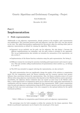
  • 3. Figure 1: Order Crossover (source: Genetic Algorithms and Genetic Programming by M. Affenzeller, S. Wagner, S. Winkler and A. Beham) • Order Crossover (OX). This crossover operator is implemented as described in the book Genetic Algorithms and Genetic Programming by M. Affenzeller, S. Wagner, S. Winkler and A. Beham. See also figure 1 and listing 12. This operator was implemented because the book described this operator as one of the better crossover operators for the TSP problem. • Sequential Constructive Crossover (SCX). This crossover operator is implemented as described in the paper Genetic Algorithm for the Traveling Salesman Problem using Sequential Constructive Crossover Operator by Zakir H. Ahmed. This crossover operator is very similar to the Heuristic Crossover as described in the book Genetic Algorithms and Genetic Programming by M. Affen- zeller, S. Wagner, S. Winkler and A. Beham. The main difference is that the SCX operates on path representation and does not randomly resolves cycles, but uses the cities that sequentially follow the current city in the path, for both parents, and then uses the heuristic (shortest dis- tance) to chose one city. Therefore, this crossover operator combines the heuristic crossover and the order crossover in one, very good operator (see also test results in the second part of the report). See also listing 13. • Edge Recombination Crossover (ERX). This crossover operator is implemented as described in the book Genetic Algorithms and Genetic Programming by M. Affenzeller, S. Wagner, S. Winkler and A. Beham. See also listing 14. This operator was implemented because it is a popular operator among other students and it is also described in the book as one of the better operators. • Heuristic Edge Recombination Crossover (Heuristic ERX). This operator is almost the same as ERX operator, except that the shortest edge from the edge map is chosen for the offspring, instead of the edge to the city with the fewest entities in its own edge list (like ERX does) or prioritizing the edges present in both parents (like Enhanced Edge Recombination Crossover (EERX) does). See also listing 15. This operator performed very well in the experiments. The Heuristic ERX and SCX operators came out as best operators from the experiments. See also the second part of the report for the experiments results. 4 Mutation operators Next to the Reciprocal Exchange and Simple Inversion mutation operators already present in the template, the following mutation operators were implemented and tested: • Insertion (position-based). This operator randomly chooses a city, removes it from the tour and inserts it at a randomly selected place. See also listing 16. • Inversion (cut-inversion). This is similar mutation operator to the inversion mutation, but it reinserts the reversed sub-tour at a random position. See also listing 17. 3
  • 4. The best operator seems to be the Simple Inversion operator (see the second part of the report for experiments results) that already was included in the template. This operator changes only two edges where the selected sub-tour has the same sequence of the visited cities, but in reverse order. Therefore, this operator introduces new genetic material with a minimal impact on the good tours and the mutation ratio can be kept high for fast converging operators like SCX and Heuristic ERX. 5 Automation of experiments For running the experiments, the following elements were implemented: • Extension of the run ga function to return the relevant results. This function was adapted to return the used parameters, best result found (distance and the tour), so that they can be written to file for later analysis when the experiment is finished. See also listing 1. • Function for running multiple experiments at once in parallel (e.g., experiment8, see also listing 18). This function runs the experiments with different parameters (random or predetermined) and writes the results in a comma separated values (csv) file for later analysis. • Work around for the Matlab string concatenation when using parallel computing. String concate- nation did not work in parallel loop, simple wrapping in a Matlab function solved this problem. See also listing 19. • Displaying of the found solution. The graphical visualisation is nod turned on when running automated experiments (this would be impossible, for example, when running several hundred experiments at once). Nevertheless, it is interesting to see some solutions found by the algorithm, a simple function was implemented for that purpose. See also listing 20. • Automated processing of the data. The resulting csv file as generated by the automated exper- iments is not easy to process manually. It contains raw data, and for example, the found best solution is not very useful for statistical analysing the data. Therefore, a Perl script was writ- ten to process the data (see also listings 21 and 22). More in particular, the script outputs the following files: – Transformed csv file in a format usable in other software, like for example R for statistical analysis. – File with computed mean distances of the found solutions. For the distances mean compu- tation, the categorical parameters (crossover, mutation and local improvement operators) are grouped (the selection method is assumed to be K-tournament with a continuous value for the K parameter and therefore it is not grouped), and for each unique combination of these parameters a mean is computed. Also, the best found solution (distance and the error percentage) are computed, together with the Mean Error Percentage for the given parameters group. This proved to be very useful for comparing the different operators, etc. – The means for the CPU time are only applicable when comparing the different selection methods and are not used in other experiments (the CPU time is not reliable when running experiments in parallel, but they are reliable when running single experiment on a single core, this became apparent after running the first set of experiments for selection methods). See also the second part of this report. – Best solution found file. This file takes the best solution found from the whole experiment and outputs the tour, the distance, the error percentage and the used parameters. – Early convergence file. This file outputs the data where the algorithm was stopped using the stop percentage, i.e., before reaching the MaxGen number of generations. The combination of the automated Matlab function with the Perl script for processing the data proved to be a very efficient way of running the experiments. The tables as shown in the second part of the report are based on the csv files processed with the Perl script. 4
  • 5. 6 GUI extension Also the GUI was extended to support all of the implemented parameters. This proved to be useful for measuring the CPU times (as the algorithm runs on a single core when executed from the GUI). For example, the results shown in the table 1 in section 1 are generated this way. Figure 2 shows a screen-shot of the extended GUI (code is not included in the appendix). Figure 2: Extended GUI Part II Experimentation and results 7 Selection methods These were the first experiments performed. The original idea was to do a kind of grid search for the best parameters. For the first experiment a minimal set of possible values was chosen (e.g., only two values: a high value and a low value): • Comparison of different selection strategies. All implemented selection strategies were going to be tested, including k-tournament with different k-values (2, 4 and 6). Ten strategies in total. • High (500) and low (100) value for the number of individuals. • High (500) and low (100) value for the number of generations. • High (0.9) and low (0.1) value for the probability of crossover. • High (0.9) and low (0.1) value for the probability of mutation. 5
  • 6. • Other parameters were fixed: stop percentage = 0.95, elitist = 0.1, crossover = xalt edges, local loop = On. • 5 iteration of each parameter settings group and 3 benchmark problems where used. • In total: 5 ∗ 3 ∗ 2 ∗ 2 ∗ 2 ∗ 2 ∗ 10 = 2400 experiments. This approach failed, as the experiments run for a very long time. Running it on multiple machines would help, but the number of experiments grows exponentially with the size of the grid; i.e., number of possible values for each parameter, therefore, even on multiple machines the running time would be very long for a more accurate experiment. In order to run the first experiment, good values for the parameters were chosen by manual experimentation (I have already tried different parameters in the exercise session, so I had an idea what could work with xalt edges operator). More methodical approach is used in later experiments (see the next section). Finally, the following experiments (among others, only the most relevant experiments are discussed) were done for the selection strategies: • Experiment 1 (see also figure 3, the tables in that figure are csv files processed with Perl script and opened in a spreadsheet processor): – 10 selection strategies – 3 problems: Belgian tour (small), benchmark with 380 cities (medium) and benchmark with 711 cities (large) – 5 runs for each combination of selection strategy/problem – the parameters: high mutation probability, low crossover probability, 500 generations, 150 individuals • Experiment 2 (see also figure 4): – since the first experiment has shown that the selection pressure is the most important factor for choosing the selection strategy, see also conclusion and interpretations below, different k values were tested (from low to very high): k = 2, 6, 10, 20, 30, 40, 60 Important conclusions and interpretations: • K-tournament seems to be a good option. It allows setting the selection pressure with the K-value and therefore can be easily used with different crossover operators that work better with low or high selection pressure. Further improvement of allowing continuous values for the K parameter made it a good choice for experimentation. • O(1) RWS was not proven. This was more a curiosity, no special attention is given to this selection method in further experiments. • Alternating edge crossover does not perform very well. The experiments were more evolutionary algorithm then genetic algorithm: the selection pressure was set very high (this even resembles hill climbing algorithm) to obtain good results, crossover rate was low and mutation rate was high. Better crossover operators were implemented for further testing. • Good experiment setup is important. With better experiment setup the running time can be reduced and good parameters can be found more easily. See also the remaining experiments. The K-tournament selection strategy is used in all remaining experiments. It proved to be very versatile, allowing turning off the selection pressure (setting the K value to 1), to setting it very high (large K values lean towards hill climbing algorithms). Further improvements of the K-tournament are also possible (e.g., adaptive K value for changing the selection pressure during the run of the algorithm), but it was not investigated. The focus of the remaining experiments was on crossover and mutation operators. 6
  • 7. Figure 3: Experiment 1. Figure 4: Experiment 2. 7
  • 8. 8 Remaining experiments For the remaining experiments, the problem with 131 cities was used (this was hard enough for all operators, as globally optimal solutions were not found, and small enough to keep the computation time limited). It is a benchmark problem with a known optimal solution, so the percentage error was used to evaluate the experiments. The experiments were also better designed, focusing on the crossover and mutation operators. The other parameters where kept in a range (determined empirically) that was big enough so the optimal value was likely included, and small enough to reduce the variation of the quality of the found solution. The parameter values were chosen at random within that range, to reduce the influence of these parameter values, allowing a good comparison of the crossover and mutation operators (the experiment results were consistent, so the statistical techniques as ANOVA or Regression did not seem to be necessary, it remains a possible improvement to the used methodology). Many experiments were performed, only the most important of them are discussed: • Experiment 3 (see also figure 5): – This experiment compares many different options: 3 crossover operators (SCX, OX and Alternating Edges), Local Improvement (on or off) and the 4 mutation operators (Insertion, Reciprocal Exchange, Inversion and Simple Inversion). As it tests different options and it is intended as a first exploration, the parameter range is large (larger variation of the found solutions). – SCX is clearly the winner of this test. The difference between the OX and Alternating Edges crossovers is less outspoken, with OX performing better than Alternating Edges. Since the SCX is by a large margin better than the other two, it is chosen for further exploration in the next experiments. – Local Improvement does not seem to be important for the SCX operator. It can be explained by that both, local improvement and SCX are heuristic operators, therefore the Local Improvement is redundant for the SCX. • Experiment 4 (see also figure 6): – This is one of the smaller experiments further exploring the influence of the local improve- ment, mutation operators and the parameters range for the SCX operator. – The SCX does not seem to have any advantage in using the local improvement, it even seems that the SCX works better without it (most likely it is due to the statistical error, however, there could be small influence by Local Improvement undoing some of the mutation changes). Since the Local Improvement also requires extra computation, it is turned off in later experiments. – The influence of the mutation operators is not clear at this stage. However, the experiments did allow for further narrowing of the parameter range. • Experiment 5 (see also figure 7): – This is a bigger experiment (960 runs of the GA) further exploring the influence of the mutation operators with a narrower range of the parameters. – It is clear that the Simple Inversion and Inversion work better than the Insertion and the Reciprocal Exchange operators. This could be explained by that the first two operators are less destructive for the tours (and sub-tours), given that the mutation rate is high enough to introduce new genetic material for the fast converging SCX operator. Best working mutation rate is around 55%. This is rather high mutation rate, this could be explained by that the heuristic operator can easily undo many of the mutations, and that the fast convergence rate of the SCX permits (or even requires) higher mutation rates. – Parameters that work well: mutation percentage around 55% (as discussed above), crossover percentage around 70% (this is quite normal rate), population around 300 (more or less 8
  • 9. twice the number of cities, this is also to be expected), around 5% elite (lower values work also well, as long as it is not 0%) and low selection pressure with K around 2 (it helps to preserve genetic diversity for fast convergence operators like SCX). The GA’s were run with 600 generations. However, SCX converges fast and tends to get stuck in a local optimum. Small improvements can be observed up to 200 generations (they still happen after that, but at very low rate). Nevertheless, the experiments were run with 600 generations, as sometimes the algorithm can get ”lucky”, as can be seen for the solution with 1.5% error. This is very low, more representative values are between 3 and 4 percent, with occasionally the error percentage dropping below 3% (it drops below 3% more easily for larger populations with many generations, see also figure 10b, error below 2% remains exceptional). Figure 5: Experiment 3. Figure 6: Experiment 4. Figure 7: Experiment 5. After running the above described experiments, I wanted to try also other operators, that I could compare with SCX. I wanted to try the ERX operator, as it was popular among other students, and 9
  • 10. it was easy to extend it with a heuristic. I have implemented the two operators (ERX and Heuristic ERX) and run the following experiment: • Experiment 6 (see also figure 8): – This is a medium experiment with 480 runs of the GA, the compared operators are the ERX and Heuristic ERX operators with Simple Inversion and Inversion mutation operators. – The parameter range is the same as in the experiment 5. This values are also close to optimal for the Heuristic ERX. However, the ERX works better with much lower mutation rate (mutation rate around 5% seems to work very well). Nevertheless, even with adapted mutation rate the error percentage remains higher for the ERX than for Heuristic ERX (best seen result was around 7%). It could be possible to optimize ERX to obtain even better results, but it seemed not necessary since it needs many generations (around 600) to obtain low error percentage, while Heuristic ERX only needs 50 generations to achieve even lower error rates, while it is also a computationally efficient operator (see the test below). – Heuristic ERX is a very good operator. The results suggest that is even better than SCX. Even if this is due to a statistical error, the ERX is computationally more efficient than SCX, making it the first choice. From the obtained results: Heuristic ERX is best, followed by SCX, ERX, OX and Alternating edges at the end. – The Simple Inversion operator was again the best from the tests, making it the best muta- tion operator among the tested operators. Figure 8: Experiment 6. In order to compare the computational times for the different crossover operators, a test was run where the parameters where kept the same for all operators, running for 200 generations and population of 300. The results are shown in table 2. From that table, it is noticeable that the ERX is a relatively fast operator, as it has an opinion of being expensive due to the need of the construction of the edge map. It is almost as fast as OX. Even the Heuristic ERX is very fast, with only a very small difference compared to the ERX. It is clear that SCX is very expensive. This numbers could be different for other programming environments than Matlab or different implementation choices. HERX is clearly the best operator that I have implemented. Test AltEdges OX SCX ERX HERX CPU 110.1591s 26.8284 170.0268s 29.3589 30.2929 Error percentage 269.7051 165.3390 6.4763 133.4527 3.9726 Table 2: Difference in computation speed between the implemented crossover operators. Figure 9 shows the best solutions as found by the SCX and HERX operators during the above described experiments (experiment 5 and 6) compared to the optimal solution for the xqf131 bench- mark problems. Figure 10 shows the results of a single-run experiments with the HERX operator for the different benchmark problems (belgiumtour, xqf131, bcl380 and rbx711). 10
  • 11. (a) SCX (1.52% error) (b) HERX (1.62% error) (c) Optimal solution Figure 9: Comparison of the solutions found in the experiments with the optimal solution. (a) belgiumtour (b) xqf131 (2.28% error) (c) bcl380 (3.97% error) (d) rbx711 (3.59% error) Figure 10: Single-run experiments for the bechmark problems. 11
  • 12. Part III Appendix: Code Listings 1 code/run ga path.m . . . . . . . . . . . . . . . . . . . . . . . . . . . . . . . . . . . . . 12 2 code/tspfun path.m . . . . . . . . . . . . . . . . . . . . . . . . . . . . . . . . . . . . . 14 3 code/tsp ImprovePopulation path.m . . . . . . . . . . . . . . . . . . . . . . . . . . . . 14 4 code/fitsc rws.m . . . . . . . . . . . . . . . . . . . . . . . . . . . . . . . . . . . . . . . 15 5 code/fitsc sus.m . . . . . . . . . . . . . . . . . . . . . . . . . . . . . . . . . . . . . . . . 15 6 code/k tournament.m . . . . . . . . . . . . . . . . . . . . . . . . . . . . . . . . . . . . 16 7 code/lin rank rws.m . . . . . . . . . . . . . . . . . . . . . . . . . . . . . . . . . . . . . 16 8 code/non lin rank rws.m . . . . . . . . . . . . . . . . . . . . . . . . . . . . . . . . . . . 17 9 code/non lin rank sus.m . . . . . . . . . . . . . . . . . . . . . . . . . . . . . . . . . . . 17 10 code/o1 rws.m . . . . . . . . . . . . . . . . . . . . . . . . . . . . . . . . . . . . . . . . 18 11 code/erx.m . . . . . . . . . . . . . . . . . . . . . . . . . . . . . . . . . . . . . . . . . . 19 12 code/cross ox.m . . . . . . . . . . . . . . . . . . . . . . . . . . . . . . . . . . . . . . . . 20 13 code/cross scx.m . . . . . . . . . . . . . . . . . . . . . . . . . . . . . . . . . . . . . . . 21 14 code/cross erx.m . . . . . . . . . . . . . . . . . . . . . . . . . . . . . . . . . . . . . . . 22 15 code/cross herx.m . . . . . . . . . . . . . . . . . . . . . . . . . . . . . . . . . . . . . . 23 16 code/insertion.m . . . . . . . . . . . . . . . . . . . . . . . . . . . . . . . . . . . . . . . 25 17 code/inversion.m . . . . . . . . . . . . . . . . . . . . . . . . . . . . . . . . . . . . . . . 25 18 code/experiment8.m . . . . . . . . . . . . . . . . . . . . . . . . . . . . . . . . . . . . . 26 19 code/add strings.m . . . . . . . . . . . . . . . . . . . . . . . . . . . . . . . . . . . . . . 28 20 code/disp sol.m . . . . . . . . . . . . . . . . . . . . . . . . . . . . . . . . . . . . . . . . 28 21 code/run.pl . . . . . . . . . . . . . . . . . . . . . . . . . . . . . . . . . . . . . . . . . . 28 22 code/transform.pl . . . . . . . . . . . . . . . . . . . . . . . . . . . . . . . . . . . . . . . 28 Listing 1: code/run ga path.m function r e s u l t = run ga path (x , y , NIND, MAXGEN, NVAR, ELITIST , STOP PERCENTAGE, PR CROSS, PR MUT, CROSSOVER, LOCALLOOP, ah1 , ah2 , ah3 , SELECTION, KVALUE, MUTATION) % usage : run ga path (x , y , % NIND, MAXGEN, NVAR, % ELITIST , STOP PERCENTAGE, % PR CROSS, PR MUT, CROSSOVER, % ah1 , ah2 , ah3 ) % % % x , y : coordinates of the c i t i e s % NIND: number of i n d i v i d u a l s % MAXGEN: maximal number of generations % ELITIST : percentage of e l i t e population % STOP PERCENTAGE: percentage of equal f i t n e s s ( stop criterium ) % PR CROSS: p r o b a b i l i t y f o r crossover % PR MUT: p r o b a b i l i t y f o r mutation % CROSSOVER: the crossover operator % c a l c u l a t e distance matrix between each pair of c i t i e s % ah1 , ah2 , ah3 : axes handles to v i s u a l i s e tsp % edited 16/11/2014 by Eryk Kulikowski : added return to the function f o r running experiments whithout gui % and changed the d ef a ul t representation to path representation {NIND MAXGEN NVAR ELITIST STOP PERCENTAGE PR CROSS PR MUT CROSSOVER LOCALLOOP SELECTION KVALUE ’ path ’ MUTATION} GGAP = 1 − ELITIST ; mean fits=zeros (1 ,MAXGEN+1) ; worst=zeros (1 ,MAXGEN+1) ; 12
  • 13. Dist=zeros (NVAR,NVAR) ; f o r i =1: s i z e (x , 1 ) f o r j =1: s i z e (y , 1 ) Dist ( i , j )=sqrt (( x( i )−x( j ) ) ˆ2+(y( i )−y( j ) ) ˆ2) ; end end % i n i t i a l i z e population Chrom=zeros (NIND,NVAR) ; f o r row=1:NIND % PATH % %Chrom(row , : )=path2adj ( randperm (NVAR) ) ; Chrom(row , : )=randperm (NVAR) ; end gen=0; % number of i n d i v i d u a l s of equal f i t n e s s needed to stop stopN=c e i l (STOP PERCENTAGE∗NIND) ; % evaluate i n i t i a l population % PATH % %ObjV = tspfun (Chrom , Dist ) ; ObjV = tspfun path (Chrom , Dist ) ; best=zeros (1 ,MAXGEN) ; % generational loop while gen<MAXGEN sObjV=sort (ObjV) ; best ( gen+1)=min(ObjV) ; minimum=best ( gen+1) ; mean fits ( gen+1)=mean(ObjV) ; worst ( gen+1)=max(ObjV) ; f o r t =1: s i z e (ObjV , 1 ) i f (ObjV( t )==minimum) break ; end end best found = Chrom( t , : ) ; % PATH % %visualizeTSP (x , y , adj2path (Chrom( t , : ) ) , minimum , ah1 , gen , best , mean fits , worst , ah2 , ObjV , NIND, ah3 ) ; visualizeTSP (x , y , Chrom( t , : ) , minimum , ah1 , gen , best , mean fits , worst , ah2 , ObjV , NIND, ah3 ) ; i f (sObjV( stopN )−sObjV (1) <= 1e −15) break ; end %assign f i t n e s s values to e n t i r e population %FitnV=ranking (ObjV) ; %s e l e c t i n d i v i d u a l s f o r breeding %SelCh=s e l e c t ( ’ sus ’ , Chrom , FitnV , GGAP) ; SelCh=f e v a l (SELECTION, Chrom , ObjV , GGAP, KVALUE) ; %recombine i n d i v i d u a l s ( crossover ) % PATH % %SelCh = recombin (CROSSOVER, SelCh ,PR CROSS, Dist ) ; PATH CROSSOVER = add strings (CROSSOVER, ’ path ’ ) ; SelCh = recombin (PATH CROSSOVER, SelCh ,PR CROSS, Dist ) ; % PATH % − see mutateTSP %SelCh=mutateTSP ( ’ inversion ’ , SelCh ,PR MUT) ; SelCh=mutateTSP path (MUTATION, SelCh ,PR MUT) ; %evaluate o f f s pr i n g , c a l l o b j e c t i v e function % PATH % %ObjVSel = tspfun ( SelCh , Dist ) ; ObjVSel = tspfun path ( SelCh , Dist ) ; %r e i n s e r t o f f s p r i n g into population [ Chrom ObjV]= r e i n s (Chrom , SelCh ,1 ,1 , ObjV , ObjVSel ) ; % PATH % − see tsp ImprovePopulation %Chrom = tsp ImprovePopulation (NIND, NVAR, Chrom ,LOCALLOOP, Dist ) ; Chrom = tsp ImprovePopulation path (NIND, NVAR, Chrom ,LOCALLOOP, Dist ) ; %increment generation counter 13
  • 14. gen=gen+1; end r e s u l t = {NIND MAXGEN NVAR ELITIST STOP PERCENTAGE PR CROSS PR MUT CROSSOVER LOCALLOOP SELECTION KVALUE gen minimum ’ path ’ MUTATION best found }; end Listing 2: code/tspfun path.m % tspfun path .m % ObjVal = tspfun path (Phen , Dist ) % Implementation of the TSP f i t n e s s function % Phen contains the phenocode of the matrix coded in path representation % Dist i s the matrix with precalculated distances between each pair of c i t i e s % ObjVal i s a vector with the f i t n e s s values f o r each candidate tour (=each row of Phen ) % % Author : Eryk Kulikowski % Date : 20−Nov−2014 function ObjVal = tspfun path (Phen , Dist ) ; ObjVal = zeros ( s i z e (Phen , 1 ) ,1) ; f o r k=1: s i z e (Phen , 1 ) ObjVal (k)=Dist (Phen(k , 1 ) ,Phen(k , s i z e (Phen , 2 ) ) ) ; f o r t = 1: s i z e (Phen , 2 )−1 ObjVal (k)=ObjVal (k)+Dist (Phen(k , t ) ,Phen(k , t+1)) ; end end end % End of function Listing 3: code/tsp ImprovePopulation path.m % tsp ImprovePopulation path .m % Author : Mike Matton % % This function improves a tsp population by removing l o c a l loops from % each i n d i v i d u a l . % % Syntax : improvedPopulation = tsp ImprovePopulation path ( popsize , n c i t i e s , pop , improve , d i s t s ) % % Input parameters : % popsize − The population s i z e % n c i t i e s − the number of c i t i e s % pop − the current population ( adjacency representation ) % improve − Improve the population (0 = no improvement , <>0 = improvement ) % d i s t s − distance matrix with distances between the c i t i e s % % Output parameter : % improvedPopulation − the new population a f t e r loop removal ( i f improve % <> 0 , e l s e the unchanged population ) . function newpop = tsp ImprovePopulation path ( popsize , n c i t i e s , pop , improve , d i s t s ) i f ( improve ) f o r i =1: popsize % PATH % %r e s u l t = improve path ( n c i t i e s , adj2path ( pop ( i , : ) ) , d i s t s ) ; r e s u l t = improve path ( n c i t i e s , pop ( i , : ) , d i s t s ) ; % PATH % %pop ( i , : ) = path2adj ( r e s u l t ) ; 14
  • 15. end end newpop = pop ; Listing 4: code/fitsc rws.m % FITSC RWS.M ( FITness SCaling Roulette Wheel S e l e c t i o n ) % % This function performs Roulette Wheel S e l e c t i o n with f i t n e s s s c a l i n g . % % Syntax : SelCh = f i t s c r w s (Chrom , ObjV , GGAP, KValue ) % % Input parameters : % Chrom − Matrix containing the i n d i v i d u a l s ( parents ) of the current % population . Each row corresponds to one i n d i v i d u a l . % ObjV − Column vector containing the o b j e c t i v e values of the % i n d i v i d u a l s in the current population ( cost values ) . % GGAP − Rate of i n d i v i d u a l s to be s e l e c t e d % i f omitted 1.0 i s assumed % KValue − ( optional ) only a pp li ca bl e f o r k−tournament s e l e c t i o n ( ignore ) % % Output parameters : % SelCh − Matrix containing the s e l e c t e d i n d i v i d u a l s . % Author : Eryk Kulikowski % Date : 16−Nov−2014 function SelCh = f i t s c r w s (Chrom , ObjV , GGAP, KValue ) % Assign f i t n e s s values to e n t i r e population Omax = max( ObjV ) ; FitnV = Omax − ObjV ; %FitnV = exp (Omax − ObjV) −1.0; % S e l e c t i n d i v i d u a l s f o r breeding SelCh=s e l e c t ( ’ rws ’ , Chrom , FitnV , GGAP) ; end % End of function Listing 5: code/fitsc sus.m % FITSC SUS .M ( FITness SCaling Stochastic Universal Sampling ) % % This function performs Stochastic Universal Sampling with f i t n e s s s c a l i n g . % % Syntax : SelCh = f i t s c s u s (Chrom , ObjV , GGAP, KValue ) % % Input parameters : % Chrom − Matrix containing the i n d i v i d u a l s ( parents ) of the current % population . Each row corresponds to one i n d i v i d u a l . % ObjV − Column vector containing the o b j e c t i v e values of the % i n d i v i d u a l s in the current population ( cost values ) . % GGAP − Rate of i n d i v i d u a l s to be s e l e c t e d % i f omitted 1.0 i s assumed % KValue − ( optional ) only a pp li ca bl e f o r k−tournament s e l e c t i o n ( ignore ) % % Output parameters : % SelCh − Matrix containing the s e l e c t e d i n d i v i d u a l s . % Author : Eryk Kulikowski % Date : 16−Nov−2014 function SelCh = f i t s c s u s (Chrom , ObjV , GGAP, KValue ) 15
  • 16. % Assign f i t n e s s values to e n t i r e population Omax = max( ObjV ) ; FitnV = Omax − ObjV ; %FitnV = exp (Omax − ObjV) −1.0; % S e l e c t i n d i v i d u a l s f o r breeding SelCh=s e l e c t ( ’ sus ’ , Chrom , FitnV , GGAP) ; end % End of function Listing 6: code/k tournament.m % KTOURNAMENT.M (K−TOURNAMENT s e l e c t i o n ) % % This function performs k tournament s e l e c t i o n . % % Syntax : SelCh = k tournament (Chrom , ObjV , GGAP, KValue ) % % Input parameters : % Chrom − Matrix containing the i n d i v i d u a l s ( parents ) of the current % population . Each row corresponds to one i n d i v i d u a l . % ObjV − Column vector containing the o b j e c t i v e values of the % i n d i v i d u a l s in the current population ( cost values ) . % GGAP − Rate of i n d i v i d u a l s to be s e l e c t e d i f omitted 1.0 i s assumed % KValue − Number of i n d i v i d u a l s p a r t i c i p a t i n g in a tournament % ( r e g u l a t e s s e l e c t i o n pressure ) % % Output parameters : % SelCh − Matrix containing the s e l e c t e d i n d i v i d u a l s . % Author : Eryk Kulikowski % Date : 15−Nov−2014 function SelCh = k tournament (Chrom , ObjV , GGAP, KValue ) % Compute number of new i n d i v i d u a l s ( to s e l e c t ) [ Nind , ans ] = s i z e ( ObjV ) ; NSel=max( f l o o r ( Nind∗GGAP+.5) ,2) ; % S e l e c t i n d i v i d u a l s f o r breeding SelCh = [ ] ; f o r i =1:NSel RowIndex = randi ( Nind ) ; K = f l o o r ( KValue ) ; pK = KValue − K; i f rand<pK K = K+1; end f o r j =1:(K − 1) RowIndex2 = randi ( Nind ) ; i f ObjV( RowIndex ) > ObjV( RowIndex2 ) ; RowIndex = RowIndex2 ; end end SelCh = [ SelCh ; Chrom(RowIndex , : ) ] ; end end % End of function Listing 7: code/lin rank rws.m % LIN RANK RWS.M ( LINear RANK RWS s e l e c t i o n ) % % This function performs Roulette Wheel S e l e c t i o n with l i n e a r ranking . % % Syntax : SelCh = lin rank rws (Chrom , ObjV , GGAP, KValue ) % 16
  • 17. % Input parameters : % Chrom − Matrix containing the i n d i v i d u a l s ( parents ) of the current % population . Each row corresponds to one i n d i v i d u a l . % ObjV − Column vector containing the o b j e c t i v e values of the % i n d i v i d u a l s in the current population ( cost values ) . % GGAP − Rate of i n d i v i d u a l s to be s e l e c t e d % i f omitted 1.0 i s assumed % KValue − ( optional ) only a pp li ca bl e f o r k−tournament s e l e c t i o n ( ignore ) % % Output parameters : % SelCh − Matrix containing the s e l e c t e d i n d i v i d u a l s . % Author : Eryk Kulikowski % Date : 16−Nov−2014 function SelCh = lin rank rws (Chrom , ObjV , GGAP, KValue ) % Assign f i t n e s s values to e n t i r e population FitnV=ranking (ObjV) ; % S e l e c t i n d i v i d u a l s f o r breeding SelCh=s e l e c t ( ’ rws ’ , Chrom , FitnV , GGAP) ; end % End of function Listing 8: code/non lin rank rws.m % NON LIN RANK RWS.M (NON LINear RANK RWS s e l e c t i o n ) % % This function performs Roulette Wheel S e l e c t i o n with non l i n e a r ranking . % % Syntax : SelCh = non lin rank rws (Chrom , ObjV , GGAP, KValue ) % % Input parameters : % Chrom − Matrix containing the i n d i v i d u a l s ( parents ) of the current % population . Each row corresponds to one i n d i v i d u a l . % ObjV − Column vector containing the o b j e c t i v e values of the % i n d i v i d u a l s in the current population ( cost values ) . % GGAP − Rate of i n d i v i d u a l s to be s e l e c t e d % i f omitted 1.0 i s assumed % KValue − ( optional ) only a pp li ca bl e f o r k−tournament s e l e c t i o n ( ignore ) % % Output parameters : % SelCh − Matrix containing the s e l e c t e d i n d i v i d u a l s . % Author : Eryk Kulikowski % Date : 16−Nov−2014 function SelCh = non lin rank rws (Chrom , ObjV , GGAP, KValue ) % Assign f i t n e s s values to e n t i r e population %RFun = [ 2 . 0 1 ] ; [ Nind , ans ] = s i z e ( ObjV ) ; RFun = exp ( l i n s p a c e (0 ,1.0986 , Nind ) ’) −1; FitnV=ranking (ObjV , RFun) ; % S e l e c t i n d i v i d u a l s f o r breeding SelCh=s e l e c t ( ’ rws ’ , Chrom , FitnV , GGAP) ; end % End of function Listing 9: code/non lin rank sus.m % NON LIN RANK SUS.M (NON LINear RANK SUS s e l e c t i o n ) % % This function performs Stochastic Universal Sampling with non l i n e a r ranking . 17
  • 18. % % Syntax : SelCh = non lin rank sus (Chrom , ObjV , GGAP, KValue ) % % Input parameters : % Chrom − Matrix containing the i n d i v i d u a l s ( parents ) of the current % population . Each row corresponds to one i n d i v i d u a l . % ObjV − Column vector containing the o b j e c t i v e values of the % i n d i v i d u a l s in the current population ( cost values ) . % GGAP − Rate of i n d i v i d u a l s to be s e l e c t e d % i f omitted 1.0 i s assumed % KValue − ( optional ) only a pp li ca bl e f o r k−tournament s e l e c t i o n ( ignore ) % % Output parameters : % SelCh − Matrix containing the s e l e c t e d i n d i v i d u a l s . % Author : Eryk Kulikowski % Date : 16−Nov−2014 function SelCh = non lin rank sus (Chrom , ObjV , GGAP, KValue ) % Assign f i t n e s s values to e n t i r e population %RFun = [ 2 . 0 1 ] ; [ Nind , ans ] = s i z e ( ObjV ) ; RFun = exp ( l i n s p a c e (0 ,1.0986 , Nind ) ’) −1; FitnV=ranking (ObjV , RFun) ; % S e l e c t i n d i v i d u a l s f o r breeding SelCh=s e l e c t ( ’ sus ’ , Chrom , FitnV , GGAP) ; end % End of function Listing 10: code/o1 rws.m % O1 RWS.M (O(1) r o u l e t t e wheel s e l e c t i o n ) % % This function performs O(1) ( constant time ) r o u l e t t e wheel s e l e c t i o n . % Based on ” Roulette−wheel s e l e c t i o n via s t o c h a s t i c acceptance ” paper % by Adam Lipowski and Dorota Lipowska . % % Syntax : SelCh = o1 rws (Chrom , ObjV , GGAP, KValue ) % % Input parameters : % Chrom − Matrix containing the i n d i v i d u a l s ( parents ) of the current % population . Each row corresponds to one i n d i v i d u a l . % ObjV − Column vector containing the o b j e c t i v e values of the % i n d i v i d u a l s in the current population ( cost values ) . % GGAP − Rate of i n d i v i d u a l s to be s e l e c t e d % i f omitted 1.0 i s assumed % KValue − ( optional ) only a pp li ca bl e f o r k−tournament s e l e c t i o n ( ignore ) % % Output parameters : % SelCh − Matrix containing the s e l e c t e d i n d i v i d u a l s . % Author : Eryk Kulikowski % Date : 15−Nov−2014 function SelCh = o1 rws (Chrom , ObjV , GGAP, KValue ) % Compute number of new i n d i v i d u a l s ( to s e l e c t ) [ Nind , ans ] = s i z e ( ObjV ) ; NSel=max( f l o o r ( Nind∗GGAP+.5) ,2) ; % Assign f i t n e s s values to e n t i r e population Omax = max( ObjV ) ; FitnV = Omax − ObjV ; %FitnV = exp (Omax − ObjV) −1.0; % S e l e c t i n d i v i d u a l s f o r breeding 18
  • 19. SelCh = [ ] ; Wmax = max( FitnV ) ; f o r i =1:NSel RowIndex = NaN; IndSelected = f a l s e ; while not ( IndSelected ) RowIndex = randi ( Nind ) ; pSelect = FitnV ( RowIndex ) /Wmax; i f pSelect > rand (1) IndSelected = true ; end end SelCh = [ SelCh ; Chrom(RowIndex , : ) ] ; end end % End of function Listing 11: code/erx.m % ERX.M ( Edge Recombination Crossover ) % % Edge Recombination Crossover as described in the book ” Genetic Algorithms and Genetic Programming” by % M. A f f e n z e l l e r , S . Wagner , S . Winkler and A. Beham . % % Syntax : NewChrom = erx (OldChrom , XOVR, Dist ) % % Input parameters : % OldChrom − Matrix containing the chromosomes of the old % population . Each l i n e corresponds to one i n d i v i d u a l % ( in any form , not n e c e s s a r i l y r e a l values ) . % XOVR − Probability of recombination occurring between p a i r s % of i n d i v i d u a l s . % Dist − the matrix with precalculated distances between each pair of c i t i e s % % Output parameter : % NewChrom − Matrix containing the chromosomes of the population % a f t e r mating , ready to be mutated and/ or evaluated , % in the same format as OldChrom . % Author : Eryk Kulikowski % Date : 13−Dec−2014 function NewChrom = erx (OldChrom , XOVR, Dist ) i f nargin < 2 , XOVR = NaN; end [ rows , c o l s ]= s i z e (OldChrom) ; maxrows=rows ; i f rem( rows , 2 ) ˜=0 maxrows=maxrows−1; end f o r row =1:2: maxrows % crossover of the two chromosomes % r e s u l t s in 2 o f f s p r i n g s i f rand<XOVR % recombine with a given p r o b a b i l i t y % PATH % %NewChrom(row , : ) =c r o s s e r x ( [ OldChrom(row , : ) ; OldChrom( row +1 ,:) ] ) ; %NewChrom( row +1 ,:)=c r o s s e r x ( [ OldChrom( row +1 ,:) ; OldChrom(row , : ) ] ) ; NewChrom(row , : )=path2adj ( c r o s s e r x ( [ adj2path (OldChrom(row , : ) ) ; adj2path (OldChrom( row +1 ,:) ) ] ) ) ; NewChrom( row +1 ,:)=path2adj ( c r o s s e r x ( [ adj2path (OldChrom( row +1 ,:) ) ; adj2path (OldChrom (row , : ) ) ] ) ) ; 19
  • 20. e l s e NewChrom(row , : )=OldChrom(row , : ) ; NewChrom( row +1 ,:)=OldChrom( row +1 ,:) ; end end i f rem( rows , 2 ) ˜=0 NewChrom( rows , : )=OldChrom( rows , : ) ; end end % End of function Listing 12: code/cross ox.m % CROSS OX.M (CROSSover operator : Order Crossover ) % % Low l e v e l function to perform recombination of two parrents into one o f f s p r i n g using the % Order Crossover as described in the book ” Genetic Algorithms and Genetic Programming” by % M. A f f e n z e l l e r , S . Wagner , S . Winkler and A. Beham % % Syntax : Offspring = cross ox ( Parents ) % % Input parameters : % Parents − Matrix containing the 2 i n d i v i d u a l s ( parents as rows ) to be recombined . % This operator assumes ”path” representation . % Dist − the matrix with precalculated distances between each pair of c i t i e s % % Output parameters : % Offspring − One row containing the constructed o f f s p r i n g i n d i v i d u a l . % Author : Eryk Kulikowski % Date : 21−Nov−2014 function Offspring = cross ox ( Parents , Dist ) ; c o l s = s i z e ( Parents , 2 ) ; Offspring = zeros (1 , c o l s ) ; parent1 = Parents ( 1 , : ) ; parent2 = Parents ( 2 , : ) ; % choose a subtour in the f i r s t parrent and copy i t to the o f f s p r i n g rndi=zeros (1 ,2) ; while rndi (1)==rndi (2) rndi=rand int ( 1 , 2 , [ 1 c o l s ] ) ; end rndi = sort ( rndi ) ; Offspring ( rndi (1) : rndi (2) ) = parent1 ( rndi (1) : rndi (2) ) ; % cancel the c i t i e s present in the subtour from the second parent f o r i=rndi (1) : rndi (2) index = find ( parent2 == Offspring ( i ) ) ; parent2 ( index ) = 0; end % i n s e r t the remaining c i t i e s from parent two into the o f f s p r i n g node = 1; f o r i =1: rndi (1)−1 while parent2 ( node )==0 node = node +1; end Offspring ( i ) = parent2 ( node ) ; node = node +1; end f o r i=rndi (2) +1: c o l s while parent2 ( node )==0 node = node +1; 20
  • 21. end Offspring ( i ) = parent2 ( node ) ; node = node +1; end end % end function Listing 13: code/cross scx.m % CROSS SCX.M (CROSSover operator : Sequential Constructive Crossover ) % % Low l e v e l function to perform recombination of two parrents into one o f f s p r i n g using the Sequential % Constructive Crossover as described in the paper ” Genetic Algorithm f o r the Traveling Salesman % Problem using Sequential Constructive Crossover Operator” by Zakir H. Ahmed. % % Syntax : Offspring = c r o s s s c x ( Parents , Dist ) % % Input parameters : % Parents − Matrix containing the 2 i n d i v i d u a l s ( parents as rows ) to be recombined . % This operator assumes ”path” representation . % Dist − the matrix with precalculated distances between each pair of c i t i e s % % Output parameters : % Offspring − One row containing the constructed o f f s p r i n g i n d i v i d u a l . % Author : Eryk Kulikowski % Date : 20−Nov−2014 function Offspring = c r o s s s c x ( Parents , Dist ) ; c o l s = s i z e ( Parents , 2 ) ; Offspring = zeros (1 , c o l s ) ; parent1 = Parents ( 1 , : ) ; parent2 = Parents ( 2 , : ) ; % node ” s t a r t i n d e x ” from parent one i s the f i r s t l e g i t i m a t e node that goes into o f s s p r i n g s t a r t i n d e x=rand int ( 1 , 1 , [ 1 c o l s ] ) ; offspringNode = parent1 ( s t a r t i n d e x ) ; Offspring (1) = offspringNode ; pcn1 = s t a r t i n d e x ; pcn2 = find ( parent2 == offspringNode ) ; f o r node = 2: c o l s % find the l e g i t i m a t e node f o r parrent 1 parent1 ( pcn1 ) = 0; parent2 ( pcn2 ) = 0; lnp1 = 0; while (( lnp1 == 0) & ( pcn1 < c o l s ) ) pcn1 = pcn1 + 1; lnp1 = parent1 ( pcn1 ) ; end i f ( lnp1 == 0) % s t a r t from the beginning of the chromosome pcn1 = 0; while ( lnp1 == 0) pcn1 = pcn1 + 1; lnp1 = parent1 ( pcn1 ) ; end end % the same f o r parrent two lnp2 = 0; while (( lnp2 == 0) & ( pcn2 < c o l s ) ) pcn2 = pcn2 + 1; lnp2 = parent2 ( pcn2 ) ; end 21
  • 22. i f ( lnp2 == 0) % s t a r t from the beginning of the chromosome pcn2 = 0; while ( lnp2 == 0) pcn2 = pcn2 + 1; lnp2 = parent2 ( pcn2 ) ; end end % choose the l g i t i m a t e node ( lnp1 or lnp2 ) with the lower distance d1 = Dist ( offspringNode , lnp1 ) ; d2 = Dist ( offspringNode , lnp2 ) ; chosenNode = lnp2 ; i f ( d2 < d1 ) chosenNode = lnp2 ; pcn1 = find ( parent1 == chosenNode ) ; e l s e chosenNode = lnp1 ; pcn2 = find ( parent2 == chosenNode ) ; end offspringNode = chosenNode ; Offspring ( node ) = offspringNode ; end end % end function Listing 14: code/cross erx.m % CROSS ERX.M (CROSSover operator : Edge Recombination Crossover ) % % Low l e v e l function to perform recombination of two parrents into one o f f s p r i n g using the Edge % Recombination Crossover as described in the book ” Genetic Algorithms and Genetic Programming” by % M. A f f e n z e l l e r , S . Wagner , S . Winkler and A. Beham % % Syntax : Offspring = c r o s s e r x ( Parents ) % % Input parameters : % Parents − Matrix containing the 2 i n d i v i d u a l s ( parents as rows ) to be recombined . % This operator assumes ”path” representation . % % Output parameters : % Offspring − One row containing the constructed o f f s p r i n g i n d i v i d u a l . % Author : Eryk Kulikowski % Date : 13−12−2014 function Offspring = c r o s s e r x ( Parents ) ; c o l s = s i z e ( Parents , 2 ) ; Offspring = zeros (1 , c o l s ) ; edgeMap = zeros (5 , c o l s ) ; f o r i = 1:2 i f (( edgeMap (1 , Parents ( i , 1 ) ) <2) | | (( edgeMap (2 , Parents ( i , 1 ) )˜=Parents ( i , c o l s ) ) && ( edgeMap (3 , Parents ( i , 1 ) )˜=Parents ( i , c o l s ) ) && (edgeMap (4 , Parents ( i , 1 ) )˜=Parents ( i , c o l s ) ) ) ) edgeMap (1 , Parents ( i , 1 ) ) = edgeMap (1 , Parents ( i , 1 ) ) + 1; edgeMap(edgeMap (1 , Parents ( i , 1 ) ) +1, Parents ( i , 1 ) ) = Parents ( i , c o l s ) ; end i f (( edgeMap (1 , Parents ( i , c o l s ) ) <2) | | (( edgeMap (2 , Parents ( i , c o l s ) )˜=Parents ( i , 1 ) ) && (edgeMap (3 , Parents ( i , c o l s ) )˜=Parents ( i , 1 ) ) && (edgeMap (4 , Parents ( i , c o l s ) )˜= Parents ( i , 1 ) ) ) ) edgeMap (1 , Parents ( i , c o l s ) ) = edgeMap (1 , Parents ( i , c o l s ) ) + 1; edgeMap(edgeMap (1 , Parents ( i , c o l s ) ) +1, Parents ( i , c o l s ) ) = Parents ( i , 1 ) ; end f o r j =1:( cols −1) 22
  • 23. i f (( edgeMap (1 , Parents ( i , j ) ) <2) | | (( edgeMap (2 , Parents ( i , j ) )˜=Parents ( i , j +1)) && (edgeMap (3 , Parents ( i , j ) )˜=Parents ( i , j +1)) && (edgeMap (4 , Parents ( i , j ) )˜=Parents ( i , j +1)) ) ) edgeMap (1 , Parents ( i , j ) ) = edgeMap (1 , Parents ( i , j ) ) + 1; edgeMap(edgeMap (1 , Parents ( i , j ) ) +1, Parents ( i , j ) ) = Parents ( i , j +1) ; end i f (( edgeMap (1 , Parents ( i , j +1)) <2) | | (( edgeMap (2 , Parents ( i , j +1))˜=Parents ( i , j ) ) && (edgeMap (3 , Parents ( i , j +1))˜=Parents ( i , j ) ) && (edgeMap (4 , Parents ( i , j +1))˜=Parents ( i , j ) ) ) ) edgeMap (1 , Parents ( i , j +1)) = edgeMap (1 , Parents ( i , j +1)) + 1; edgeMap(edgeMap (1 , Parents ( i , j +1)) +1, Parents ( i , j +1)) = Parents ( i , j ) ; end end end % choose s t a r t c i t y index=rand int ( 1 , 1 , [ 1 c o l s ] ) ; Offspring (1) = index ; f o r i =2: c o l s c i t y = 0; nbEdges = 5; f o r j =1:edgeMap (1 , index ) i f (edgeMap (1 , edgeMap( j +1, index ) ) ˜= 0) i f (edgeMap (1 , edgeMap( j +1, index ) ) < nbEdges ) c i t y = edgeMap( j +1, index ) ; nbEdges = edgeMap (1 , edgeMap( j +1, index ) ) ; e l s e i f (edgeMap (1 , edgeMap( j +1, index ) ) == nbEdges && rand <0.5) c i t y = edgeMap( j +1, index ) ; nbEdges = edgeMap (1 , edgeMap( j +1, index ) ) ; end end end i f c i t y == 0 u n v i s i t e d C i t i e s = zeros (1 , c o l s ) ; nbuc = 0; f o r k=1: c o l s i f (( edgeMap (1 , k) ˜= 0)&&(k˜=index ) ) nbuc=nbuc+1; u n v i s i t e d C i t i e s ( nbuc )=k ; end end c i t y=u n v i s i t e d C i t i e s ( rand int ( 1 , 1 , [ 1 nbuc ] ) ) ; end edgeMap (1 , index ) =0; Offspring ( i ) = c i t y ; index = c i t y ; end end % end function Listing 15: code/cross herx.m % CROSS HERX.M (CROSSover operator : H e u r i s t i c Edge Recombination Crossover ) % % Low l e v e l function to perform recombination of two parrents into one o f f s p r i n g using the H e u r i s t i c Edge % Recombination Crossover . % % Syntax : Offspring = cross herx ( Parents ) % % Input parameters : % Parents − Matrix containing the 2 i n d i v i d u a l s ( parents as rows ) to be recombined . % This operator assumes ”path” representation . % Dist − the matrix with precalculated distances between each pair of c i t i e s % % Output parameters : 23
  • 24. % Offspring − One row containing the constructed o f f s p r i n g i n d i v i d u a l . % Author : Eryk Kulikowski % Date : 17−12−2014 function Offspring = cross herx ( Parents , Dist ) ; c o l s = s i z e ( Parents , 2 ) ; Offspring = zeros (1 , c o l s ) ; edgeMap = zeros (5 , c o l s ) ; f o r i = 1:2 i f (( edgeMap (1 , Parents ( i , 1 ) ) <2) | | (( edgeMap (2 , Parents ( i , 1 ) )˜=Parents ( i , c o l s ) ) && ( edgeMap (3 , Parents ( i , 1 ) )˜=Parents ( i , c o l s ) ) && (edgeMap (4 , Parents ( i , 1 ) )˜=Parents ( i , c o l s ) ) ) ) edgeMap (1 , Parents ( i , 1 ) ) = edgeMap (1 , Parents ( i , 1 ) ) + 1; edgeMap(edgeMap (1 , Parents ( i , 1 ) ) +1, Parents ( i , 1 ) ) = Parents ( i , c o l s ) ; end i f (( edgeMap (1 , Parents ( i , c o l s ) ) <2) | | (( edgeMap (2 , Parents ( i , c o l s ) )˜=Parents ( i , 1 ) ) && (edgeMap (3 , Parents ( i , c o l s ) )˜=Parents ( i , 1 ) ) && (edgeMap (4 , Parents ( i , c o l s ) )˜= Parents ( i , 1 ) ) ) ) edgeMap (1 , Parents ( i , c o l s ) ) = edgeMap (1 , Parents ( i , c o l s ) ) + 1; edgeMap(edgeMap (1 , Parents ( i , c o l s ) ) +1, Parents ( i , c o l s ) ) = Parents ( i , 1 ) ; end f o r j =1:( cols −1) i f (( edgeMap (1 , Parents ( i , j ) ) <2) | | (( edgeMap (2 , Parents ( i , j ) )˜=Parents ( i , j +1)) && (edgeMap (3 , Parents ( i , j ) )˜=Parents ( i , j +1)) && (edgeMap (4 , Parents ( i , j ) )˜=Parents ( i , j +1)) ) ) edgeMap (1 , Parents ( i , j ) ) = edgeMap (1 , Parents ( i , j ) ) + 1; edgeMap(edgeMap (1 , Parents ( i , j ) ) +1, Parents ( i , j ) ) = Parents ( i , j +1) ; end i f (( edgeMap (1 , Parents ( i , j +1)) <2) | | (( edgeMap (2 , Parents ( i , j +1))˜=Parents ( i , j ) ) && (edgeMap (3 , Parents ( i , j +1))˜=Parents ( i , j ) ) && (edgeMap (4 , Parents ( i , j +1))˜=Parents ( i , j ) ) ) ) edgeMap (1 , Parents ( i , j +1)) = edgeMap (1 , Parents ( i , j +1)) + 1; edgeMap(edgeMap (1 , Parents ( i , j +1)) +1, Parents ( i , j +1)) = Parents ( i , j ) ; end end end % choose s t a r t c i t y index=rand int ( 1 , 1 , [ 1 c o l s ] ) ; Offspring (1) = index ; f o r i =2: c o l s c i t y = 0; d = 0; f o r j =1:edgeMap (1 , index ) i f (edgeMap (1 , edgeMap( j +1, index ) ) ˜= 0) d2 = Dist ( index , edgeMap( j +1, index ) ) ; i f (d==0) c i t y = edgeMap( j +1, index ) ; d = d2 ; e l s e i f (d>d2 ) c i t y = edgeMap( j +1, index ) ; d = d2 ; end end end i f c i t y == 0 d = 0; f o r k=1: c o l s i f (( edgeMap (1 , k) ˜= 0)&&(k˜=index ) ) d2 = Dist ( index , k) ; i f (d==0) c i t y = k ; d = d2 ; e l s e i f (d>d2 ) c i t y = k ; d = d2 ; 24
  • 25. end end end end edgeMap (1 , index ) =0; Offspring ( i ) = c i t y ; index = c i t y ; end end % end function Listing 16: code/insertion.m % INSERTION.M (INSERTION mutation ) % % This low l e v e l function performs I n s e r t i o n mutation operator . This operator s e l e c t s a % city , removes i t and r e i n s e r t s at random point . % % Syntax : NewChrom = i n s e r t i o n (OldChrom , Representation ) % % Input parameters : % OldChrom − Vector containing the i n d i v i d u a l to be mutated . % Representation − Representation i s an i n t e g e r s p e c i f y i n g which encoding i s used % 1 : adjacency representation % 2 : path representation % % Output parameters : % NewChrom − Vector containing the mutated i n d i v i d u a l . % Author : Eryk Kulikowski % Date : 21−Nov−2014 function NewChrom = i n s e r t i o n (OldChrom , Representation ) ; NewChrom=OldChrom ; i f Representation==1 NewChrom=adj2path (NewChrom) ; end % s e l e c t two p o s i t i o n s in the tour % f i r s t p o s i t i o n rand (1) i s the i n s e r t i o n point , the second p o s i t i o n i s s e l e c t e d c i t y rndi=zeros (1 ,2) ; while rndi (1)==rndi (2) rndi=rand int ( 1 , 2 , [ 1 s i z e (NewChrom, 2 ) ] ) ; end %rndi = sort ( rndi ) ; i f rndi (1)<rndi (2) b u f f e r = NewChrom( rndi (2) ) ; NewChrom( rndi (1) +1: rndi (2) ) = NewChrom( rndi (1) : rndi (2) −1) ; NewChrom( rndi (1) )=b u f f e r ; e l s e b u f f e r = NewChrom( rndi (2) ) ; NewChrom( rndi (2) : rndi (1) −1) = NewChrom( rndi (2) +1: rndi (1) ) ; NewChrom( rndi (1) )=b u f f e r ; end i f Representation==1 NewChrom=path2adj (NewChrom) ; end end % End of function 25
  • 26. Listing 17: code/inversion.m % INVERSION.M (INVERSION mutation ) % % This low l e v e l function performs Inversion mutation operator . This operator s e l e c t s a % subtour , removes it , i n v e r s e s i t and then r e i n s e r t s at random point . % % Syntax : NewChrom = i n v e r s i o n (OldChrom , Representation ) % % Input parameters : % OldChrom − Vector containing the i n d i v i d u a l to be mutated . % Representation − Representation i s an i n t e g e r s p e c i f y i n g which encoding i s used % 1 : adjacency representation % 2 : path representation % % Output parameters : % NewChrom − Vector containing the mutated i n d i v i d u a l . % Author : Eryk Kulikowski % Date : 21−Nov−2014 function NewChrom = i n v e r s i o n (OldChrom , Representation ) ; NewChrom=OldChrom ; i f Representation==1 NewChrom=adj2path (NewChrom) ; end % s e l e c t two p o s i t i o n s in the tour rndi=zeros (1 ,2) ; while rndi (1)==rndi (2) rndi=rand int ( 1 , 2 , [ 1 s i z e (NewChrom, 2 ) ] ) ; end rndi = sort ( rndi ) ; ins = rand int ( 1 , 1 , [ 1 s i z e (NewChrom, 2 ) −(rndi (2)−rndi (1) ) ] ) ; sub = NewChrom( rndi (2) : −1: rndi (1) ) ; i f ins==rndi (1) NewChrom( rndi (1) : rndi (2) ) = sub ; e l s e i f ins<rndi (1) b u f f e r = NewChrom( ins : rndi (1) −1) ; NewChrom( ins : ins+rndi (2)−rndi (1) ) = sub ; NewChrom( ins+rndi (2)−rndi (1) +1: rndi (2) ) = b u f f e r ; e l s e b u f f e r = NewChrom( rndi (2) +1: ins+rndi (2)−rndi (1) ) ; NewChrom( ins : ins+rndi (2)−rndi (1) ) = sub ; NewChrom( rndi (1) : ins −1) = b u f f e r ; end i f Representation==1 NewChrom=path2adj (NewChrom) ; end end % End of function Listing 18: code/experiment8.m % EXPERIMENT8.M % % Help function to perform experiments in a p a r a l l e l s e t t i n g ( using parfor ) . % Several experiments can be run with d i f f e r e n t parameters , the r e s u l t s are written in a cvs f i l e . 26
  • 27. % Author : Eryk Kulikowski % Date : 18−Nov−2014 function experiment8 () ; ah1 = NaN; ah2 = NaN; ah3 = NaN; STOP PERCENTAGE = 0 . 9 9 ; number experiments = 480; FILENAME={ ’ xqf131 . tsp ’ }; sFILENAME = 1; % s i z e of FILENAME %NIND = rand int (1 , number experiments , [ 1 0 0 300]) ; %MAXGEN = rand int (1 , number experiments , [ 1 0 0 300]) ; NIND = rand int (1 , number experiments , [ 2 5 0 350]) ; MAXGEN = [ ones (1 , number experiments ) ∗ 6 0 0 ] ; ELITIST = rand (1 , number experiments ) /10; % between 0 and 10% PR CROSS = 0.6+ rand (1 , number experiments ) /3;%between 60−93.3% PR MUT = 0.5+ rand (1 , number experiments ) /10;%between 50−60% %CROSSOVER = { ’ xalt edges ’ ’ scx ’ ’ ox ’ } ; %X = [ ones (1 , number experiments /3) ones (1 , number experiments /3) ∗2 ones (1 , number experiments /3) ∗ 3 ] ; CROSSOVER = { ’ scx ’ }; X = [ ones (1 , number experiments ) ] ; %[ ans , shuf ] = sort ( rand (1 , number experiments ) ) ; %X = X( shuf ) ; %LOCALLOOP = [ ones (1 , number experiments /2) zeros (1 , number experiments /2) ] ; LOCALLOOP = [ zeros (1 , number experiments ) ] ; %[ ans , shuf ] = sort ( rand (1 , number experiments ) ) ; %LOCALLOOP = LOCALLOOP( shuf ) ; SELECTION = { ’ k tournament ’ }; S = [ ones (1 , number experiments ) ] ; KVALUE = rand (1 , number experiments ) ∗5 +1; MUTATION = { ’ i n s e r t i o n ’ ’ rexchange ’ }; M = [ ones (1 , number experiments /2) ones (1 , number experiments /2) ∗ 2 ] ; [ ans , shuf ] = sort ( rand (1 , number experiments ) ) ; M = M( shuf ) ; s t r = s p r i n t f ( ’%s ,%s ,%s ,%s ,%s ,%s ,%s ,%s ,%s ,%s ,%s ,%s ,%s ,%s ,%s ,%s ,%s n ’ , ’NIND ’ , ’MAXGEN ’ , ’NVAR’ , ’ELITIST ’ , ’STOP PERCENTAGE’ , . . . ’PR CROSS ’ , ’PR MUT’ , ’CROSSOVER’ , ’LOCALLOOP’ , ’SELECTION ’ , ’KVALUE’ , ’ gen ’ , ’ minimum ’ , ’ cpu time ’ , ’ representation ’ , ’ mutation ’ , ’ best found ’ ) ; z = 0; % 10 experiments f o r each set of values to know avarage and standard deviation parfor i = 1: number experiments f o r f = 1:sFILENAME data = load ( [ ’ datasets / ’ FILENAME{ f } ] ) ; %x=data ( : , 1 ) /max ( [ data ( : , 1 ) ; data ( : , 2 ) ] ) ; %y=data ( : , 2 ) /max ( [ data ( : , 1 ) ; data ( : , 2 ) ] ) ; x=data ( : , 1 ) ; y=data ( : , 2 ) ; NVAR=s i z e ( data , 1 ) ; %[ x y ] = i n p u t c i t i e s (NVAR) ; started = t i c ; r e s u l t = run ga path (x , y , NIND( i ) , MAXGEN( i ) , NVAR, ELITIST( i ) , STOP PERCENTAGE, PR CROSS( i ) , . . . PR MUT( i ) , CROSSOVER{X( i ) } , LOCALLOOP( i ) , ah1 , ah2 , ah3 , SELECTION{S( i ) } , KVALUE( i ) , MUTATION{M( i ) }) ; f i n i s h e d = toc ( started ) s = ’ ’ ; best found = r e s u l t {16}; f o r j =1: s i z e ( best found , 2 ) s = add strings ( s , s p r i n t f ( ’%d ’ , best found ( j ) ) ) ; end s ( end ) = [ ] ; 27
  • 28. str2 = s p r i n t f ( ’%d,%d,%d,%.2 f ,%.2 f ,%.2 f ,%.2 f ,%s ,%d,%s ,%.2 f ,%d,%.6 f ,%.6 f ,%s ,%s ,[% s ] n ’ , r e s u l t {1} , r e s u l t {2} , r e s u l t {3} , r e s u l t {4} , . . . r e s u l t {5} , r e s u l t {6} , r e s u l t {7} , r e s u l t {8} , r e s u l t {9} , r e s u l t {10} , r e s u l t {11} , r e s u l t {12} , r e s u l t {13} , finished , r e s u l t {14} , r e s u l t {15} , s ) ; s t r = add strings ( str , str2 ) ; z = z + 1 end end f i l e I D = fopen ( ’ /path/ to / experiments / f o l d e r / experiment . csv ’ , ’w ’ ) ; f p r i n t f ( f ileID , ’%s ’ , s t r ) ; f c l o s e ( f i l e I D ) ; end Listing 19: code/add strings.m % ADD STRINGS.M % % Help function to concatenate two s t r i n g s in p a r a l l e l s e t t i n g ( using parfor ) . % Author : Eryk Kulikowski % Date : 16−Nov−2014 function s t r = add strings ( str1 , str2 ) s t r = s p r i n t f ( ’%s%s ’ , str1 , str2 ) ; end Listing 20: code/disp sol.m % d i s p s o l .M % % Help function to v i s u a l i z e the found s o l u t i o n . % Author : Eryk Kulikowski % Date : 22−Nov−2014 function d i s p s o l ( DatasetFile , TotalDist , Solution ) data = load ( [ ’ datasets / ’ DatasetFile ] ) ; x=data ( : , 1 ) ; y=data ( : , 2 ) ; NVAR=s i z e ( data , 1 ) ; fh = f i g u r e ( ’ V i s i b l e ’ , ’ o f f ’ , ’Name ’ , ’TSP Tool ’ , ’ Position ’ ,[0 ,0 ,1024 ,768]) ; ah1 = axes ( ’ Parent ’ , fh , ’ Position ’ , [ . 1 .1 .8 . 8 ] ) ; plot (x , y , ’ ko ’ ) axes ( ah1 ) ; plot (x( Solution ) ,y( Solution ) , ’ ko−’ , ’ MarkerFaceColor ’ , ’ Black ’ ) ; hold on ; plot ( [ x( Solution ( length ( Solution ) ) ) x( Solution (1) ) ] , [ y( Solution ( length ( Solution ) ) ) y( Solution (1) ) ] , ’ ko−’ , ’ MarkerFaceColor ’ , ’ Black ’ ) ; t i t l e ( [ ’ Beste rondrit lengte : ’ num2str ( TotalDist ) ] ) ; hold o f f ; drawnow ; end Listing 21: code/run.pl #!/ usr / bin / perl system ( ” perl transform . pl experiment . csv cpu . csv means . csv best . txt early . csv exp data . csv ” ) ; e x i t (0) ; Listing 22: code/transform.pl #!/ usr / bin / perl 28
  • 29. # transform . pl # Compute the mean values f o r the experiments . # param 1: o r i g i n a l csv data # param 2: cpu times means # param 3: minimum distance means # param 4: best s o l u t i o n found output f i l e # param 5: early convergence f i l e # param 6: transformed CSV data # Author : Eryk Kulikowski use s t r i c t ; use warnings ; # open the o r i g i n a l data open FILE , ”<” , $ARGV[ 0 ] or die $ ! ; # skip the header l i n e my $ l i n e = <FILE>; # prepare the output f i l e s : ec and transformed open ECFILE, ”>” , $ARGV[ 4 ] or die $ ! ; open OUTFILE, ”>” , $ARGV[ 5 ] or die $ ! ; # write the new header #”NIND,MAXGEN,NVAR, ELITIST ,STOP PERCENTAGE,PR CROSS,PR MUT,CROSSOVER,LOCALLOOP, SELECTION,KVALUE, gen , minimum , cpu time , representation , mutation , best found n” print ECFILE ”Nind , Maxgen , Elit , Pc ,Pm, SelPress , Crossover , Mutation , LocalImpr ,Minumum, PercErr , Genn” ; print OUTFILE ”Nind , Maxgen , Elit , Pc ,Pm, SelPress , Crossover , Mutation , LocalImpr ,Minumum, PercErr , Genn” ; # mean vars my %parameter comb ;# counter − mean my %s e l e c t i o n c p u ;# counter − mean # best s o l u t i o n s found vars my $minimum value ; my $minimum pe ; my $minimum line ; # i t e r a t e over the l i n e s containing the data , ” ,” separated while ( $ l i n e = <FILE>) { # chop the n chop ( $ l i n e ) ; my @line data = s p l i t (/ ,/ , $ l i n e ) ; #NIND=0,MAXGEN=1,NVAR=2,ELITIST=3,STOP PERCENTAGE=4,PR CROSS=5,PR MUT=6,CROSSOVER=7 #LOCALLOOP=8,SELECTION=9,KVALUE=10,gen=11,minimum=12, cpu time =13, representation =14 #mutation=15, found solution =16 my $parameters = ” $ l i n e d a t a [ 7 ] $ l i n e d a t a [ 1 5 ] $ l i n e d a t a [ 8 ] ” ;#f o r the minimum mean my $ s e l e c t i o n = ” $ l i n e d a t a [ 7 ] $ l i n e d a t a [ 1 5 ] $ l i n e d a t a [ 8 ] ” ;#f o r the cpu mean my $nvar = $ l i n e d a t a [ 2 ] ; my $nind = $ l i n e d a t a [ 0 ] ; my $maxgen = $ l i n e d a t a [ 1 ] ; my $ e l i t = $ l i n e d a t a [ 3 ] ; my $pc = $ l i n e d a t a [ 5 ] ; my $pm = $ l i n e d a t a [ 6 ] ; my $ s e l p r e s s = $ l i n e d a t a [ 1 0 ] ; my $cross = $ l i n e d a t a [ 7 ] ; my $mut = $ l i n e d a t a [ 1 5 ] ; my $locimp ; i f ( $ l i n e d a t a [ 8 ] == 0) { $locimp = ” Off ” ;} e l s e { $locimp = ”On” ;} my $minimum = $ l i n e d a t a [ 1 2 ] ; my $cpu time = $ l i n e d a t a [ 1 3 ] ; my $gen = $ l i n e d a t a [ 1 1 ] ; #global minimum my $global minimum ; $global minimum = 564 i f ( $nvar == 131) ; 29
  • 30. $global minimum = 1621 i f ( $nvar == 380) ; $global minimum = 2513 i f ( $nvar == 662) ; $global minimum = 3115 i f ( $nvar == 711) ; $global minimum = 0 unless ( defined ( $global minimum ) ) ; #percentage e r r o r my $pe ; i f ( $global minimum != 0) {$pe = 100∗($minimum/$global minimum − 1) ;} e l s e {$pe = ”NaN” ;} #”Nind , Maxgen , Elit , Pc ,Pm, SelPress , Crossover , Mutation , LocalImpr ,Minumum, PercErr , Genn” print OUTFILE ”$nind , $maxgen , $ e l i t , $pc ,$pm, $selpress , $cross , $mut , $locimp , $minimum , $pe , $genn” ; i f ( $gen < $maxgen ) { print ECFILE ”$nind , $maxgen , $ e l i t , $pc ,$pm, $selpress , $cross , $mut , $locimp , $minimum , $pe , $genn” ; } # means i f ( defined ( $parameter comb{ $parameters }) ) { $parameter comb{ $parameters } [ 0 ] ++; $parameter comb{ $parameters } [ 1 ] += $minimum ; i f ( $parameter comb{ $parameters } [ 2 ] > $minimum) { $parameter comb{ $parameters } [ 2 ] = $minimum ; } } e l s e { # i n s e r t values my @a = (1 , $minimum , $minimum , $global minimum ) ; $parameter comb{ $parameters } = @a; } i f ( defined ( $minimum value ) ) { i f ($minimum < $minimum value ) { $minimum value = $minimum ; $minimum pe = $pe ; $minimum line = $ l i n e ; } } e l s e { $minimum value = $minimum ; $minimum pe = $pe ; $minimum line = $ l i n e ; } i f ( defined ( $ s e l e c t i o n c p u { $ s e l e c t i o n }) ) { $ s e l e c t i o n c p u { $ s e l e c t i o n }[0]++; $ s e l e c t i o n c p u { $ s e l e c t i o n } [ 1 ] += $cpu time ; } e l s e { my @a = (1 , $cpu time ) ; $ s e l e c t i o n c p u { $ s e l e c t i o n } = @a; } } c l o s e (FILE) ; c l o s e (ECFILE) ; c l o s e (OUTFILE) ; #cpu times # make 2D array from hash my @cpu times ; my $counter = 0; foreach my $k ( keys %s e l e c t i o n c p u ) { $cpu times [ $counter ] [ 0 ] = $k ; $cpu times [ $counter ] [ 1 ] = $ s e l e c t i o n c p u {$k } [ 0 ] ; $cpu times [ $counter ] [ 2 ] = $ s e l e c t i o n c p u {$k } [ 1 ] ; $counter++; } # sort @cpu times = sort { $$a [ 2 ] <=> $$b [ 2 ] } @cpu times ; open OUTFILE, ”>” , $ARGV[ 1 ] or die $ ! ; print OUTFILE ” Crossover Mutation LocalImpr , cpu time meann” ; f o r my $i (0..$# cpu times ) 30
  • 31. { my $mean = $cpu times [ $i ] [ 2 ] / $cpu times [ $i ] [ 1 ] ; print OUTFILE ” $cpu times [ $i ] [ 0 ] , $meann” ; } c l o s e (OUTFILE) ; # means # make 2D array from hash my @means ; $counter = 0; foreach my $k ( keys %parameter comb ) { $means [ $counter ] [ 0 ] = $k ; $means [ $counter ] [ 1 ] = $parameter comb{$k } [ 0 ] ; $means [ $counter ] [ 2 ] = $parameter comb{$k } [ 1 ] ; $means [ $counter ] [ 3 ] = $parameter comb{$k } [ 2 ] ; $means [ $counter ] [ 4 ] = $parameter comb{$k } [ 3 ] ; $counter++; } # sort @means = sort { $$a [ 2 ] <=> $$b [ 2 ] } @means ; open OUTFILE, ”>” , $ARGV[ 2 ] or die $ ! ; #”NIND,MAXGEN,NVAR, ELITIST ,STOP PERCENTAGE,PR CROSS,PR MUT,CROSSOVER,LOCALLOOP, SELECTION,KVALUE, gen , minimum , cpu time n” print OUTFILE ” Crossover Mutation LocalImpr , minimum mean ,MPE, minimum best , b e s t p e r c e r r n” ; f o r my $i (0..$# means ) { my $mean = $means [ $i ] [ 2 ] / $means [ $i ] [ 1 ] ; i f ( $means [ $i ] [ 4 ] != 0) { my $mpe = 100∗($mean/$means [ $i ] [ 4 ] −1) ; my $bpe = 100∗( $means [ $i ] [ 3 ] / $means [ $i ] [ 4 ] − 1) ; print OUTFILE ”$means [ $i ] [ 0 ] , $mean , $mpe , $means [ $i ] [ 3 ] , $bpen” ; } e l s e { print OUTFILE ”$means [ $i ] [ 0 ] , $mean ,NA, $means [ $i ] [ 3 ] ,NAn” ; } } c l o s e (OUTFILE) ; # best s o l u t i o n s found (3 tours ) open OUTFILE, ”>” , $ARGV[ 3 ] or die $ ! ; print OUTFILE ”Best s o l u t i o n s found : n” ; print OUTFILE ”Minimum = $minimum value , Percentage e r r o r = $minimum pe , s e t t i n g s : n” ; print OUTFILE ”NIND,MAXGEN,NVAR, ELITIST ,STOP PERCENTAGE,PR CROSS,PR MUT,CROSSOVER, LOCALLOOP,SELECTION,KVALUE, gen , minimum , cpu time , representation , mutation , found solution n” ; print OUTFILE ”$minimum linen” ; c l o s e (OUTFILE) ; e x i t (0) ; 31