The document discusses statistical representation of random inputs in continuum models. It provides examples of representing random fields using the Karhunen-Loeve expansion, which expresses a random field as the sum of orthogonal deterministic basis functions and random variables. Common choices for the covariance function in the expansion include the radial basis function and limiting cases of fully correlated and uncorrelated fields. The covariance function can be approximated from samples of the random field to enable representation in applications.

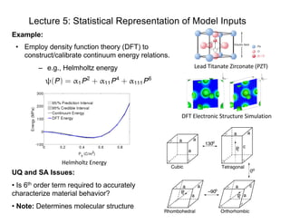
1. Lecture 5: Statistical Representation of Model Inputs
Example:
Lead Titanate Zirconate (PZT)
DFT Electronic Structure Simulation
Helmholtz Energy
(P) = ↵1P2
+ ↵11P4
+ ↵111P6
UQ and SA Issues:
• Is 6th order term required to accurately
characterize material behavior?
• Note: Determines molecular structure
• Employ density function theory (DFT) to
construct/calibrate continuum energy relations.
– e.g., Helmholtz energy
0o
P0
P0
a
aa
c
a a
Cubic Tetragonal
P0
a
a
a
Rhombohedral
a
a c
130
Orthorhombic
o
−90o

2. Quantum-Informed Continuum Models
DFT Electronic Structure Simulation
Broad Objective:
• Use UQ/SA to help bridge scales
from quantum to system
Lead Titanate Zirconate (PZT)
(P) = ↵1P2
+ ↵11P4
+ ↵111P6
UQ and SA Issues:
• Is 6th order term required to accurately
characterize material behavior?
• Note: Determines molecular structure
Objectives:
• Employ density function theory (DFT) to
construct/calibrate continuum energy relations.
– e.g., Helmholtz energy
Helmholtz Energy
Note:
• Linearly parameterized

3. Example 2: Pressurized Water Reactors (PWR)
Models:
•Involve neutron transport, thermal-hydraulics, chemistry.
•Inherently multi-scale, multi-physics.
CRUD Measurements: Consist of low resolution images at limited number of locations.

4. Thermo-Hydraulic Equations: Mass, momentum and energy balance for fluid
Challenges:
• Codes can have 15-30 closure relations and up to 75 parameters.
• Codes and closure relations often ”borrowed” from other physical phenomena;
e.g., single phase fluids, airflow over a car (CFD code STAR-CCM+)
• Calibration necessary and closure relations can conflict.
• Inference of random fields requires high- (infinite-) dimensional theory.
Notes:
• Similar relations for gas
and bubbly phases
• Surrogate models must
conserve mass, energy,
and momentum
• Many parameters are
spatially varying and
represented by random
fields
@
@t
(↵f ⇢f ) + r · (↵f ⇢f vf ) = -
↵f ⇢f
@vf
@t
+ ↵f ⇢f vf · rvf + r · R
f + ↵f r · + ↵f rpf
= -FR
- F + (vf - vg)/2 + ↵f ⇢f g
@
@t
(↵f ⇢f ef ) + r · (↵f ⇢f ef vf + Th) = (Tg - Tf )H + Tf f
-Tg(H - ↵gr · h) + h · rT - [ef + Tf (s⇤
- sf )]
-pf
✓
@↵f
@t
+ r · (↵f vf ) +
⇢f
◆
Pressurized Water Reactors (PWR)

5. Representation of Random Inputs
Example 1: Consider the Helmholtz energy
(P) = ↵1P2
+ ↵11P4
+ ↵111P6
with frequency-dependent random parameters
(P, !, f) = ↵1(f, !)P2
+ ↵11(f, !)P4
+ ↵111(f, !)P6
Challenge 1: Difficult to work with probabilities associated with random events
! 2 ⌦.
Solution: Every realization ! 2 ⌦ yields a value q 2 Q ⇢ . Work in image of
Challenge 2: How do we represent random fields; e.g.,
↵1(f, !) – that are infinite-dimensional?
Solution: Develop a representation and approximation framework
probability space ( , B( ), ⇢(q)) instead of (⌦, F, P).

6. Example and Motivation
Example 2: Heat equation
Motivation: Consider
@⇢
@t
= ↵
@2
⇢
@x2
, 0 < x < L , t > 0
⇢(t, 0) = ⇢(t, L) = 0 t > 0
T(0, x) = ⇢0(x) 0 < x < L
@T
@t
=
@
@x
✓
↵(x, !)
@T
@x
◆
+ f(t, x) , -1 < x < 1, t > 0
T(t, -1, !) = T`(!) , T(t, 1, !) = Tr (!) t > 0
T(0, x, !) = T0(!) - 1 < x < 1

7. Example and Motivation
Motivation: Consider
@⇢
@t
= ↵
@2
⇢
@x2
, 0 < x < L , t > 0
⇢(t, 0) = ⇢(t, L) = 0 t > 0
T(0, x) = ⇢0(x) 0 < x < L
Separation of Variables: Take
Then
X 00
(x) - cX(x) = 0
X(0) = X(L) = 0
and
˙T(t) = c↵T(t)
) T(t) = ec↵t
Note: Heat decays – Mathematical argument
If c > 0, this implies that X(x) = k = 0.
Thus c < 0 so we take c = - 2
where > 0.
ZL
0
[XX 00
- cX2
]dx = -
ZL
0
⇥
(X 0
)2
+ cX2
⇤
dx = 0

8. Motivation
Boundary Value Problem:
X 00
(x) - cX(x) = 0
X(0) = X(L) = 0
Solution: X(x) = A cos( x) + B sin( x)
X(0) = 0 ) A = 0
X(L) = 0 ) L = n⇡
Thus
Xn(x) = Bn sin( nx) , n =
n⇡
L
, Bn 6= 0
Initial Condition:
⇢(t, x) =
1X
n=1
Bne-↵ 2
nt
sin( nx)
General Solution:
⇢0(x) = ⇢(0, x) =
1X
n=1
Bn sin( nx)
)
ZL
0
⇢0(x) sin( mx)dx =
ZL
0
1X
n=1
Bn sin( nx) sin( mx)dx
) Bn =
2
L
ZL
0
⇢0(x) sin( nx)dx

9. Motivation
Boundary Value Problem:
X 00
(x) - cX(x) = 0
X(0) = X(L) = 0
Initial Condition:
⇢(t, x) =
1X
n=1
Bne-↵ 2
nt
sin( nx)
General Solution:
Example: ⇢0(x) = sin
⇣⇡x
L
⌘
Bn =
2
L
ZL
0
⇢0(x) sin( nx)dx
Bn =
2
L
ZL
0
sin
⇣⇡x
L
⌘
sin
⇣n⇡x
L
⌘
dx
=
2
L
· L
2
, n = 1
0 , n 6= 1
Note Decay!
L
General Solution:
⇢(t, x) = e-↵(⇡/L)2
t
sin(⇡x/L)

10. Random Field Representation
Random Fields: Strategy – Represent random field in terms of mean
function and covariance function
↵(x, !)
↵(x)
Finite-Dimensional:
V =
2
6
6
6
6
4
var(X1) cov(X1, X2) · · ·
cov(X2, X1) var(X2)
...
...
var(Xp)
3
7
7
7
7
5
Note: Infinite-dimensional for functions
Examples: Short versus long-range interactions
Note:
Limiting Behavior:
D = [-1, 1]
c(x, y)
1. c(x, y) = 2
e-|x-y|/L
(i) L ! 1 ) c(x, y) = 1 Fully correlated so cannot truncated
(ii) L ! 0 ) c(x, y) = (x - y) Uncorrelated so easy to truncate
normalizes

11. Random Field Representation
Examples:
Gaussian
1-D Wiener Process
• Used to model Brownian motion
• Can solve eigenvalue problem explicitly
Properties of c(x,y):
1. Finite-dimensional: e.g., C = V symmetric and positive definite
C = ⇤ -1
= ⇤ T
=
2
6
4 1
· · · p
3
7
5
2
6
4
1
...
p
3
7
5
2
6
4
1
...
p
3
7
5
=
⇥
1
1
, ... , p
p
⇤
2
6
4
1
...
p
3
7
5 =
p
X
p=1
n
n
( n
)T
2. c(x, y) = min(x, y)
3. c(x, y) = 2
e-(x-y)2
/2L2
MATLAB: covariance_exp.m, covariance_min.m, covariance_Gaussian.m

12. Random Field Representation
Mercer’s Theorem: (Infinite Dimensional) – If c(x,y) is symmetric and positive
definite, it can be expressed as
where
and
Z
D
n(x) m(x)dx = mn
Karhunen-Loeve Expansion:
↵(x, !) = ¯↵(x) +
1X
n=1
p
n n(x)Qn(!)
Note: Eigenfunctions are orthonormal
c(x, y) =
1X
n=1
n n(x) n(y)
Z
D
c(x, y) n(y)dy = n n(x) for x 2 D

13. Random Field Representation
Karhunen-Loeve Expansion:
↵(x, !) = ¯↵(x) +
1X
n=1
p
n n(x)Qn(!)
Statistical Properties: Take
↵(x, !) = ¯↵(x) + (x, !)
(x, !) =
1X
n=1
p
n n(x)Qn(!)
) (x, !) (y, !) =
1X
n=1
1X
m=1
Qn(!)Qm(!)
p
n m n(x) m(y)
Recall: For random variables X,Y
cov(X, Y] = E[XY] - E[X]E[Y]
Notation: E[Y] = hYi =
Z
y⇢(y)dy
where (x, !) has zero mean and covariance function c(x, y). Take

14. Random Field Representation
Statistical Properties: Because (x, !) has zero mean,
Since eigenfunctions are orthogonal,
Multiplication by `(x) and integration yields
k
Z
D
k (x) `(x)dx =
1X
n=1
hQn(!)Qk (!)i
p
n k n`
) k k` =
p
k ` hQk (!)Q`(!)i
Note:
k = ` ) hQk (!)Q`(!)i = 1
k 6= ` ) hQk (!)Q`(!)i = 0
) hQk (!)Q`(!)i = k`
c(x, y) = E[ (x, !) (y, !)]
= h (x, !) (y, !)i
=
1X
n=1
1X
m=1
hQn(!)Qm(!)i
p
n m n(x) m(y)
k k (x) =
Z
D
c(x, y) k (y)dy
=
1X
n=1
hQn(!)Qk (!)i
p
n k n(x)

15. Random Field Representation
where
Karhunen-Loeve Expansion:
↵(x, !) = ¯↵(x) +
1X
n=1
p
n n(x)Qn(!)
Result: The random variables satisfy
(i) E[Qn] = 0
(ii) E[QnQm] = mn
Zero mean
Mutually orthogonal and uncorrelated
Question: How do we choose c(x,y) and compute solutions to
Z
D
c(x, y) n(y)dy = n n(x) for x 2 D
Z
D
c(x, y) n(y)dy = n n(x) for x 2 D

16. Common Choices for c(x,y)
1. Radial Basis Function:
so
Note: L is correlation length, which
quantifies smoothness or relation
between values of x and y.
Analytic Solution:
n =
2L
1+L2w2
n
, if n is even,
2L
1+L2v2
n
, if n is odd,
n(x) =
8
>><
>>:
sin(wnx)
q
1- sin(2wn)
2wn
, if n is even,
cos(vnx)
q
1+ sin(2vn)
2vn
, if n is odd
Note: wn and vn are the solutions of the transcendental equations
Lw + tan(w) = 0 , for even n,
1 - Lv tan(v) = 0 , for odd n
Z1
-1
e-|x-y|/L
n(y)dy = n n(x)
c(x, y) = e-|x-y|/L
, D = [-1, 1]

17. Common Choices for c(x,y)
1. Radial Basis Function:
so
Note: L is correlation length
Limiting Cases:
Recall:
Then
Take
n(x) = n n(x)
) n = 1 for all n
Note: Because uncorrelated,
we cannot truncate series!
Z
D
n(y)dy = n n(x) = kn
1(x) = 1(y) =
p
2
2
1 = 2
n = 0 for n = 2, 3, ...
(i) c(x, y) = 1 Fully correlated (L ! 1)
c(x, y) = 1 =
1X
n=1
n n(x) n(y)
(ii) c(x, y) = (x - y) Uncorrelated (L ! 0)
c(x, y) = e-|x-y|/L
, D = [-1, 1]
Z1
-1
e-|x-y|/L
n(y)dy = n n(x)

18. Construction of c(x,y)
Question: If we know underlying distribution can we approximate the
covariance function c(x,y)? Yes … via sampling!
! 2 ⌦,
Example: Consider the Helmholtz energy
↵(P, !) = ↵1(!)P2
+ ↵11(!)P4
+ ↵111(!)P6
and take x = P for x = P 2 [0, 1]
Note: Assume we can evaluate for various polarizations and
values from the underlying distribution
↵(xj , !k
) xj = Pj
!k
Required Steps:
• Approximation of the covariance function c(x,y)
• Approximation of the eigenvalue problem
with
Z
D
n(x) m(x)dx = mn
Z
D
c(x, y) n(y)dy = n n(x) for x 2 D

19. Construction of c(x,y)
Step 1: Approximation of covariance function c(x,y)
For NMC Monte Carlo samples !k
, covariance function approximated by
where the centered field is
↵c(x, !k
) = ↵(x, !k
) - ↵(x)
and the mean is
¯↵(x) ⇡
1
NMC
NMCX
j=1
↵(x, !j
)
c(x, y) ⇡ cNMC
(x, y) =
1
NMC - 1
NMCX
k=1
↵c(x, !k
)↵c(y, !k
)

20. Construction of c(x,y)
Step 2 (Nystrom’s Method): Approximate eigenvalue problem
with
Z
D
n(x) m(x)dx = mn
Z
D
c(x, y) n(y)dy = n n(x) for x 2 D
Consider composite quadrature rule with Nquad points and weights {(xj , wj )}.
Discretized Eigenvalue Problem:
Nquad
X
j=1
c(xi , xj ) n(xj )wj = n n(xi ) , i = 1, ... , Nquad
Matrix Eigenvalue Problem:
CW n = n n
where
i
n = n(xi )
Cij = c(xi , xj )
W = diag(w1, ... , wNquad
)
Symmetric Matrix Eigenvalue Problem:
W1/2
CW1/2 en = n
en
where
W1/2
= diag(
p
w1, ... ,
p
wNquad
)
eT
n
en = 1 ) T
n W 1 = 1
en = W1/2
n ) n = W-1/2 en

21. Algorithm to Approximate c(x,y)
Inputs:
(i) Quadrature formula with nodes and weights {(xj , wj )}
(ii) Functions evaluations {↵(xj , !k
)} , j = 1, ... , Nquad , k = 1, ... , NMc
Output: Eigenvalues, eigenvectors and KL modes
(1) Center the process
↵c(xi , !k
) = ↵(xi , !k
) -
1
NMC
NMCX
j=1
↵(xi , !j
)
for i = 1, ... , Nquad and k = 1, ... , NMC.
2) Form covariance matrix C = [Cij ] that discretizes covariance function c(x, y)
Cij =
1
NMC - 1
NMCX
k=1
↵c(xi , !k
)↵c(xj , !k
)
for i, j = 1, ... , Nquad .

22. Algorithm to Approximate c(x,y)
Output: Eigenvalues, eigenvectors and KL modes
(3) Let W = diag(w1, ... , wNquad
) and solve
W1/2
Cw1/2 en = n
en
for n = 1, ... , Nquad .
(4) Compute the eigenvectors n = W-1/2 en.
(5) Exploit the decay in the eigenvalues n to choose a KL truncation level NKL
and compute discretized KL modes Qn(!). Consider
↵(x, !) ⇡ ¯↵(x) +
NKLX
n=1
p
n n(x)Qn(!)
) ↵c(x, !) ⇡
NKLX
n=1
p
n n(x)Qn(!)
) Qn(!) =
1
p
n
Z
D
↵c(x, !) n(x)dx
⇡
1
p
n
Nquad
X
j=1
wj ↵c(xj , !) j
n.
(1)

23. Algorithm to Approximate c(x,y)
Output: Eigenvalues, eigenvectors and KL modes
(6) Sample !k
and construct surrogate eQn(!k
); e.g., polynomial, spectral poly-
nomial, Gaussian process.
Example: Consider the Helmholtz energy
↵(x, !) = ↵1(!)x2
+ ↵11x4
+ ↵111x6
for x 2 [0, 1]
Mean Values: Based on DFT
¯↵1 = -389.4 , ¯↵11 = 761.3 , ¯↵111 = 61.5.
Distribution:
↵ = [↵1, ↵11, ↵111] ⇠ U([↵1`, ↵1r ] ⇥ [↵2`, ↵2r ] ⇥ [↵3`, ↵3r ])
where ↵1` = ¯↵1 - 0.2 ¯↵1, ↵1r = ¯↵ + 0.2 ¯↵1 with similar intervals for ↵11 and ↵111
Eigenvalues: 1 = 417.88, 2 = 1.2 and 3 = 0.009 so truncate series at NKL = 3
MATLAB: covariance_construct.m

24. Example and Motivation
Example 2: Heat equation
Note: Well-posedness requires
Take
@T
@t
=
@
@x
✓
↵(x, !)
@T
@x
◆
+ f(t, x) , -1 < x < 1, t > 0
T(t, -1, !) = T`(!) , T(t, 1, !) = Tr (!) t > 0
T(0, x, !) = T0(!) - 1 < x < 1
0 < ↵min 6 ↵(x, !) 6 ↵max
↵(x, !) = ↵min + e ¯↵(x)+
P1
n=1
p
n n(x)Qn(!)
Parameters: Q = [T`, TR, T0, Q1, ... , QN ]