The document summarizes a numerical analysis of fatigue for a connecting rod in an internal combustion engine. It describes the finite element analysis methodology, including defining the 3D model, loads, meshing, and solving. Stress results are presented for two load cases: maximum compression at 1800 RPM and maximum tension at 2625 RPM. A fatigue life prediction is performed using the stress-life method and Goodman diagram. The lowest fatigue factor of 1.32 was above the acceptable limit of 1.3, indicating no expected fatigue failures under these loads.

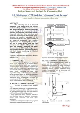
1. S B Chikalthankar, V M Nandedkar, Surendra Prasad Baratam / International Journal of
Engineering Research and Applications (IJERA) ISSN: 2248-9622 www.ijera.com
Vol. 2, Issue 6, November- December 2012, pp.628-632
Fatigue Numerical Analysis for Connecting Rod
S B Chikalthankar*, V M Nandedkar**, Surendra Prasad Baratam*
*(Department of Mechanical Engineering, Government College of Engineering, and Aurangabad)
** (SGGS Institute of Engineering and Technology, Nanded, India)
ABSTRACT
The connecting rod is a structural
component cyclic loaded during the Internal
Combustion Engines (ICE) operation, it means
that fatigue phenomena should be taken into
account during the development, in order to
guarantee the connecting rod required lifetime.
Numerical tools have been extremely used
during the connecting rod development phase,
therefore, the complete understand of the
mechanisms involved as well as the reliability of
the numerical methodology are extremely
important to take technological advantages,
such as, to reduce project lead time and
prototypes cost reduction. The present work
shows the complete connecting rod Finite
Element Analysis (FEA) methodology. It was
also performed a fatigue study based on Stress
Life (SxN) theory, considering the Modified
Goodman diagram.
Keywords – Crank System Kinematics, Fatigue
analysis, FEA Figure 1 – Connecting rod development phases
I. INTRODUCTION III. CRANK SYSTEM KINEMATICS
During the ICE operation, the connecting The connecting rod function is to link the
rod is cyclic loaded due to the engine physics piston and the crankshaft, transforming the
behavior. Basically, the tensile and compressive reciprocating movement of the piston in a rotative
forces are applied on the connecting rod during the movement of the crankshaft. The complete
engine cycle. The tensile force is applied during the knowledge of the ICE loads is important to design
exhaust stroke, while the compression occurs at the structural components such as connecting rods,
power stroke. Depending on these loads bearings and crankshafts.
magnitudes and its combination, localized cracks
can be nucleated. Adding the fact of the high cycles
presented on the ICE, premature and catastrophic
failures can occur. The intention is to present the
connecting rod FEA methodology as well as the
fatigue treatment based on SxN assumption.
II. FINITE ELEMNT METHODOLY
The FEA is divided in three different
steps:
- Pre processor: Includes the 3D model preparation,
loads and boundary condition definition, to select
the appropriated element type and shape function
and Finite Element (FE) mesh generation.
- Solver: Definition of the numerical method to
solve the linear system of equations, convergence
criteria, error estimation and strain stress
calculation.
- Post Processor: Engineers analysis and judgment Figure 2 – Scheme of conrod – crankshaft
phase based on stabilished design criteria. mechanisms
628 | P a g e

2. S B Chikalthankar, V M Nandedkar, Surendra Prasad Baratam / International Journal of
Engineering Research and Applications (IJERA) ISSN: 2248-9622 www.ijera.com
Vol. 2, Issue 6, November- December 2012, pp.628-632
Where: neglected, and thus the final equation that
L = Connecting rod length represents the piston displacement is:
r = Crank radius
θ = Crank angle
(5)
β = Connecting rod angle
x = Piston instantaneous position The instantaneous velocity can be directly obtained
TDC = Top dead center by differentiating the equation 5
The piston instantaneous position can be
calculated according to the scheme presented in
Figure 2.
Thus, we have:
(1)
(6)
Rewriting the expression:
(2) The piston acceleration can be determined by:
The equation 2 has two degrees of
freedom, but it is possible to obtain the angle β in Therefore:
terms of angle θ. (7)
Therefore: IV. DYNAMIC LOADS
The connecting rod dynamic load
calculation is determined based on the cylinder gas
Denominating λ as the relation between pressure versus crank angle curve (Figure 3), and
the crank radius ® and the connecting rod length the inertia forces generated due to the reciprocating
(L) we have: masses and the engine speed (Figure 4). The
combination of the gas force, generated due to the
cylinder gas pressure, and the inertia force, provide
Through the first trigonometry law we have: the resultant force applied on the connecting rod
(Figure 5).The conventional connecting rod
structural analysis has been performed considering
(3)
Therefore: the over load and over speed operational
conditions.
Historically, these regimes are the
(4) responsible for the maximum tensile force and
The equation 4 can be approximated by maximum compressive force respectively.
the relation: However, a combination of cylinder gas pressure
and engine speed for the intermediate operational
conditions may provide critical loads for the
connecting rod. Therefore, the complete engine
operational conditions map evaluation is
recommended in order do not omit important loads.
Therefore:
Naming a=1, we will
have:
Performing the transformations we will have:
The values of λ are usually small,
Figure 3 – Cylinder gas pressure versus crank angle
therefore the series high order terms can be
629 | P a g e

3. S B Chikalthankar, V M Nandedkar, Surendra Prasad Baratam / International Journal of
Engineering Research and Applications (IJERA) ISSN: 2248-9622 www.ijera.com
Vol. 2, Issue 6, November- December 2012, pp.628-632
The gas force can be calculated for each crank (10)
angle according to the expression bellow:
V. FINITE ELEMENT MODEL
Where: A FEA was performed in order to obtain
= Gas force at crank angle θ the connecting rod strain and stress results. In order
to simulate the connecting rod structural behavior,
= Cylinder gas pressure at crank the complete connecting rod assembly should be
angle θ taken into account, therefore, the piston pin,
D = Piston diameter bushing, bearings, crank pin and bolts should be
The inertia force is calculated by the following considered in the FE model.
expression: Historically, most connecting rod fatigue
(9) failures occur at the small end region, due to this
fact, the present study will be concentrated in this
Where
region. Therefore, the connecting rod joint surface
= Inertia force will be considered completely bonded without bolts
= Reciprocating masses and the bearings are also omitted in this analysis.
a = piston acceleration The FEA was performed using ANSYS software.
Figure 6 – Connecting rod model for FEA.
Figure 4 – Inertia force versus crank angle.
MODEL INFORMATION:
Element Type Number of elements
SOLID
6388
TETRAHEDRAL
CONTACT 77
Table 1 – FEA model information.
VI. BOUNDARY CONDITIONS
As described previously, there are two
critical loads for each engine operating condition,
the tensile force generated due to inertia, and
compressive force due to the gas load. The work
presents the FEA results performed for over load @
1800 rpm and over speed @ 2625 rpm conditions.
Figure 5 – Connecting rod resultant force.
After calculating the gas and inertia
forces, the resultant connecting rod force can be
directly determined by the expression:
630 | P a g e

4. S B Chikalthankar, V M Nandedkar, Surendra Prasad Baratam / International Journal of
Engineering Research and Applications (IJERA) ISSN: 2248-9622 www.ijera.com
Vol. 2, Issue 6, November- December 2012, pp.628-632
Figure 7 – Connecting rod load cases.
Figure 9 –Maximum principal stress @ 2625 rpm.
Over Load @1800
Over Speed @2625
rpm The figures 8 and 9 show the stress
distribution for the compressive load @ 1800 rpm
and the tensile load @2625 rpm respectively.
Table 2 - Load cases summary VIII. FATIGUE LIFE PREDICTION
The Stress Life (SxN) theory was
VII. STRESS RESULTS employed to evaluate the connecting rod fatigue
The connecting rod assembly was life. It implicates that the component will have
numerically simulated by FEA in order to evaluate infinite life for a number of cycles over to 107,
the maximum and minimum loads, according to according to.
described previously. The prestress due to press fit
assembly was also considered in all simulated
cases.
Figure 10 – Typical SxN diagram
In order to perform the fatigue study, the
finite element results should be combined to obtain
the alternate and mean stresses for each operating
condition, according to the definition bellow:
Figure 8 – Maximum principal stress @ 1800 rpm.
Figure 11 – Nomenclature for constant amplitude
cyclic loading.
631 | P a g e

5. S B Chikalthankar, V M Nandedkar, Surendra Prasad Baratam / International Journal of
Engineering Research and Applications (IJERA) ISSN: 2248-9622 www.ijera.com
Vol. 2, Issue 6, November- December 2012, pp.628-632
Based on the figure above, we can define:
(11)
(12)
Where
= Alternative stress
= Mean stress
= Maximum stress Table 3 – FEA stress results
= Minimum stress Fatigue Factors
0˚ 90˚ 180˚
Over load 4.33 2.24 1.73
The alternate and mean stresses were
Over speed 11.93 1.32 1.46
calculated for each operating condition, combining
the finite element results according to explained
below: Table 4 – Calculated fatigue factors.
According to table 4, the lowest fatigue
factor obtained was 1.32 (90º small end region).
The KMCL fatigue factor acceptable criteria is 1.3.
By analyzing the numerical results and established
acceptable criteria, we can conclude that no
After calculating the alternate and mean connecting rod fatigue failures are expected for
stresses, we can plot the Modified Goodman these loads level.
diagram.
IX. CONCLUSIONS
According to obtained results, the highest
stresses were observed in the small end region and
fatigue factors calculated for most critical nodes at
three different positions at the small end. Lowest
fatigue factor obtained was 1.32 in acceptable
range, So we can verified that the proposed
numerical methodology to evaluate the connecting
rod structural and fatigue lifetime. Therefore the
methodology presented in this work, showed to be
an important tool to be applied during the
connecting rod development phase.
REFERENCES
[1] Brunetti F., Garcia O., 1992, Motores de
Combustão Interna, FEI.
[2] ANSYS 10.0 – Release Documentation,
ANSYS Inc.
[3] Timoshenko S., 1976, Strength of Material
Vol.2, Krieger Pub Co.
Figure 12 – Modified Goodman diagram. [4] Fuchs H.O., 1980, Metal Fatigue in
Where: Engineering, A Willey-Interscience
Su = Ultimate strength Publication.
Sy = Yield strength [5] Shygley J.E., Mischke C.R., Budynas
Se = Endurance limit R.G., 2003, Mechanical Engineering
With the alternate and mean stresses, and Design, McGraw Hill.
using the Modified Goodman diagram for the [6] Lipson C., Sheth N.J., Statistical Design
connecting rod material, it is possible to evaluate and Analysis of Engineering Experiments,
the fatigue factors. Based on FEA results, the McGraw Hill.
highest stresses were observed in the small end
region, therefore, the fatigue factors were
calculated for the most critical nodes in three
different positions at the small end.
632 | P a g e