Cp34550555

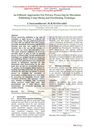
C.Saravanabhavan, Dr.R.M.S.Parvathi/ International Journal of Engineering Research and
Applications (IJERA) ISSN: 2248-9622 www.ijera.com
Vol. 3, Issue 4, Jul-Aug 2013, pp.550-555
550 | P a g e
An Efficient Approaches For Privacy Preserving In Microdata
Publishing Using Slicing and Partitioning Technique
C.Saravanabhavan1, Dr.R.M.S.Parvathi2
1Research Scholar &Asst Professor, Department of CSE, Kongunadu College of Engineering &
Technology, Tamil Nadu, India.
2Principal & Professor, Department of CSE, Sengunthar College of Engineering, Tamil Nadu, India
Abstract
Privacy preserving publishing is the kind of
techniques to apply privacy to collected vast
amount of data. The data publication processes
are today still very difficult. Data often contains
personally identifiable information and therefore
releasing such data may result in privacy
breaches; this is the case for the examples of
micro data, e.g., census data and medical data.
This paper proposed techniques to accelerate
accessing speed of user as well as applying
privacy to collected data. Several anonymization
techniques were designed for privacy preserving
data publishing. Recent work in data publishing
has shown that generalization loses considerable
amount of information, especially for high
dimensional data. Bucketization, on the other
hand, does not prevent membership disclosure.
We propose the overlapping slicing methods for
handling high-dimensional data. By partitioning
attributes into more than one column, we protect
privacy by breaking the association of
uncorrelated attributes and preserve data utility
by preserving the association between highly
correlated attributes. This technique releases
more attribute correlations. That overlapping
slicing preserves better data utility than
generalization and is more effective than
bucketization in workloads involving the
sensitive attribute.
Keyword: Data Publishing, Microdata,
Generalization, Bucketization, Anonymization.
I. Introduction
1.1 Privacy Preserving Data Publishing
In the information age, data are increasingly being
collected and used. Much of such data are person
specific, containing record for each individual.
Forexample, microdataare collected andused by
various government agencies (e.g.,U.S.Census
Bureau and Department of Motor Vehicles) and by
many commercial companies (e.g., health
organizations, insurance companies, andretailers).
Other examples include personal search histories
collected by web search engines. Companies and
agencies that collect such data often need to publish
and share the data for research and other purposes.
However, such data usually contains personal
sensitive information, the disclosure of which may
violate the individual’sprivacy. Examples of re-cent
attacks include discovering the medical diagnosis of
the governor of Massachusetts, identifying the
search history of an AOL searcher, andde-an
onymizing the movie ratings of 500,000 subscribers
of Netflix.
In the wake of the sewell publicized attacks, privacy
has become an important problem in data publishing
and data sharing. This thesis focuses on how to
publish and shared at aina privacy-preserving
manner.
1.2 Micro data Publishing
In this thesis, consider micro data such as census
data and medical data. Typically, micro data are
stored in a table, and each record (row) corresponds
to one individual. Each record has a number of
attributes, which can be divided in to the following
three categories:
1.Identifier.
Identifiers are attributes that clearly identify
individuals. Examples include Social Security
Number and Name.
Name Zip-code Age Disease
Alice 47677 29 HeartDiseas
e
Bob 47602 22 HeartDiseas
e
Carl 47678 27 HeartDiseas
e
David 47905 43 Flu
Eva 47909 52 HeartDiseas
e
Frank 47906 47 Cancer
Glory 47605 30 HeartDiseas
e
Harry 47673 36 Cancer
Table 1.1
Microdata Table (Example of Microdata)

551 | P a g e
2. Quasi-Identifier. Quasi-identifiers are attributes
whose values when taken together can potentially
identify an individual. Examples include Zip-code,
Birthdate, and Gender. An adversary may already
know the QI values of some individuals in the data.
This knowledge can be either from personal contact
or from other publicly- available databases (e.g., a
voter registration list) that include both explicit
identifiers and quasi-identifiers.
3. Sensitive Attribute. Sensitive attributes are
attributes whose values should not be associated
with an individual by the adversary. Examples
include Disease and Salary.
An example of microdata table is shown in Table
1.1. As in most previous work, assume that each
attribute in the microdata is associated with one of
the above threeattribute types and attribute types can
be specified by the data publisher.
1.2.1 Information Disclosure Risks
When releasing microdata, it is necessary
to prevent the sensitive information of the
individuals from being disclosed. Three types of
information disclosure have been identified in the
literature: membership disclosure, identity
disclosure, and attribute disclosure.
Membership Disclosure: When the data to be
published is selected from a larger population and
the selection criteria are sensitive (e.g., when
publishing datasets about diabetes patients for
research purposes), it is important to prevent an
adversary from learning whether an individual’s
record is in the data or not.
Identity Disclosure: Identity disclosure (also called
re-identification) occurs when an individual is
linked to a particular record in the released data.
Identity disclosure is what the society views as the
clearest form of privacy violation. If one is able to
correctly identify one individual’s record from
supposedly anonymized data, then people agree that
privacy is violated. In fact, most publicized privacy
attacks are due to identity disclosure. In the case of
GIC medical database, Sweeney re-identified the
medical record of the state governor of
Massachusetts. In the case of AOL search data, the
journalist from New York Times linked AOL
searcher NO. 4417749 to Thelma Arnold, a 62-year-
old widow living in Lilburn, GA. And in the case of
Netflix prize data, researchers demonstrated that an
adversary with a little bit of knowledge about an
individual subscriber can easily identify this
subscriber’s record in the data. When identity
disclosure occurs, also say “anonymity” is broken.
Attribute Disclosure:
Attribute disclosure occurs when new information
about some individuals is revealed, i.e., the released
data makes it possible to infer the characteristics of
an individual more accurately than it would be
possible before the data release. Identity disclosure
often leads to attribute disclosure. Once there is
identity disclosure, an individual is re-identified and
the corresponding sensitive values are revealed.
Attribute disclosure can occur with or without
identity disclosure. It has been recognized that even
disclosure of false attribute information may cause
harm. An observer of the released data may
incorrectly perceive that an individual’s sensitive
attribute takes a particular value, and behave
accordingly based on the perception. This can harm
the individual, even if the perception is incorrect.
In some scenarios, the adversary is assumed to know
who is and who is not in the data, i.e., the
membership information of individuals in the data.
The adversary tries to learn additional sensitive
information about the individuals. In these
scenarios, our main focus is to provide identity
disclosure protection and attribute disclosure
protection. In other scenarios where membership
information is assumed to be unknown to the
adversary membership disclosure should be
prevented. Protection against membership disclosure
also helps to protect against identity disclosure and
attribute disclosure: it is in general hard to learn
sensitive information about an individual if you
don’t even know whether this individual’s record is
in the data or not.
1.2.2 Data Anonymization
While the released data gives useful
information to researchers, it presents disclosure risk
to the individuals whose data are in the data.
Therefore, our objective is to limit the disclosure
risk to an acceptable level while maximizing the
benefit. This is achieved by anonymizing the data
before release. The first step of anonymization is to
remove explicit identifiers. However, this is not
enough, as an adversary may already know the
quasi- identifier values of some individuals in the
table. This knowledge can be either from personal
knowledge (e.g., knowing a particular individual in
person), or from other publicly- available databases
(e.g., a voter registration list) that include both
explicit identifiers and quasi-identifiers. Privacy
attacks that use quasi-identifiers to re-identify an
individual’s record from the data are also called re-
identification attacks.
To prevent re-identification attacks, further
anonymization is required. A common approach is
generalization, which replaces quasi-identifier
values with values that are less- specific but

552 | P a g e
semantically consistent. For example, age 24 can be
generalized to an age interval [20-29]. As a result,
more records will have the same set of quasi-
identifier values. Define a QI group to be a set of
records that have the same values for the quasi-
identifiers.
In other words, a QI group consists of a set of
records that are indistinguishable from each other
from their quasi-identifiers. In the literature, a QI
group is also called an “anonymity group” or an
“equivalence class.
1.3 Anonymization Framework
This section gives an overview of the problems
studied in this thesis. (1) Privacy models: what
should be the right privacy requirement for data
publishing? (2) Anonymization methods: how can
the data are anonymized to satisfy the privacy
requirement? (3) Data utility measures: how to
measure the utility of the anonymized data?
1.3.1 Privacy Models
A number of privacy models have been proposed in
the literature, including k-anonymity and ℓ -
diversity.
k-Anonymity”: Samarati and Sweeney introduced
k-anonymityas the property that each record is
indistinguishable with at least k-1other records with
respect to the quasi-identifier. In other words, k-
anonymity requires that each QI group contains at
least k records. For example, Table 1.3 is an
anonymized version of the original microdata table
in Table 1.2. And Table 1.3 satisfies 3-anonymity.
The protection k-anonymity provides is simple and
easy to understand. If a table satisfies k-anonymity
for some value k, then anyone who knows only the
quasi-identifier values of one individual cannot
identify the record corresponding to that individual
with confidence greater than 1/k.
ZIPCode Age Disease
1 47677 29 HeartDisease
4 47905 43 Flu
6 47906 47 Cancer
8 47673 36 Cancer
9 47607 32 Cancer
Table 1.2
Original Table (Example of k-anonymity)
1
ZIPCode
476**
Age
2*
Disease
HeartDisease
2 476** 2* HeartDisease
4 4790* ≥40 Flu
5 4790* ≥40 HeartDisease
6 4790* ≥40 Cancer
8 476** 3* Cancer
9 476** 3* Cancer
Table 1.3
A 3-Anonymous Table (Example of k-Anonymity)
Example 1.3.1 Consider the original patients table
in Table 1.2 and the 3-anonymous table in Table
1.3. The Disease attribute is sensitive. Suppose
Alice knows that Bob is a 27-year old man living in
ZIP 47678 and Bob’s record is in the table. From
Table 1.3, Alice can conclude that Bob corresponds
to one of the first three records, and thus must have
heart disease. This is the homogeneity attack. For
an example of the background knowledge attack,
suppose that, by knowing Carl’s age and zip code,
Alice can conclude that Carl corresponds to a record
in the last QI group in Table 1.3. Furthermore,
suppose that Alice knows that Carl has very low risk
for heart disease. This background knowledge
enables Alice to conclude that Carl most likely has
cancer.
To address these limitations of k-anonymity,
alternative approaches have been proposed. These
include discernibility, ℓ -diversity.
Definition 1.3.1 (The ℓ -diversity Principle) A QI
group is said to have ℓ -diversity if there are at least
ℓ “well-represented” values for the sensitive

553 | P a g e
attribute. A table is said to have ℓ -diversity if every
QI group of the table has ℓ -diversity.
A number of interpretations of the term “well-
represented” are given:
1. Distinct ℓ -diversity: The simplest understanding
of “well represented” would be to ensure there are at
least ℓ distinct values for the sensitive attribute in
each QI group. Distinct ℓ -diversity does not prevent
probabilistic inference attacks. A QI group may
have one value appear much more frequently than
other values, enabling an adversary to conclude that
an entity in the QI group is very likely to have that
value. This motivated the development of the
following stronger notions of ℓ -diversity.
2. Probabilistic ℓ -diversity”: An anonymized table
satisfies probabilistic ℓ -diversity if the frequency of
a sensitive value in each group is at most 1/ℓ . This
guarantees that an observer cannot infer the
sensitive value of an individual with probability
greater than 1/ℓ .
3. Entropy ℓ -diversity: The entropy of a QI group
E is defined to be in which S is the
domain of the sensitive attribute, and p(E, s) is the
fraction of records in E that have sensitive value s.
A table is said to have entropy l-diversity if for
every QI group E, Entropy (E)≥ logl. Entropy l-
diversity is strong than distinct l-diversity. As
pointed out, in order to have entropy l-diversity for
each group, the entropy of the entire table must be at
least log (l). Sometimes this may too restrictive, as
the entropy of the entire table may be low if a few
values are very common. This leads to the following
less conservation notion of l-diversity.
4. Recursive (c, ℓ )-diversity: Recursive (c, ℓ )-
diversity makes sure that the most frequent value
does not appear too frequently, and the less frequent
values do not appear too rarely. Let m be the number
of values in a QI group, and ri, 1≤ i ≤ m be the
number of times that the ith
most frequent sensitive
value appears in a QI group E. Then E is said to
have recursive (c,l)-diversity if r1< c(rl+rl+1 +…+rm).
A table is said to have recursive (c,l)-diversity if all
of its equivalence classes have recursive (c,l)-
diversity.
There are a few variants of the l- diversity model,
including p-sensitive k-anonymity and (α , k)-
Anonymity.
1.3.2 Anonymization Methods
In this section, several popular anonymization
methods are studied (also known as recoding
techniques).
Generalization and Suppression: In their seminal
work, Samarati and Sweeney proposed to use
generalization and suppression. Generalization
replaces a value with a “less-specific but
semantically consistent” value. Tuple suppression
removes an entire record from the table. Unlike
traditional privacy protection techniques such as
data swapping and adding noise, information in a k-
anonymized table through generalization and
suppression
remains truthful. For example, through
generalization, Table 1.3 is an anonymized version
of the original microdata table in Table 1.2. And
Table 1.3 satisfies 3-anonymity.
Typically, generalization utilizes a value
generalization hierarchy (VGH) for each attribute.
In a VGH, leaf nodes correspond to actual attribute
values, and internal nodes represent less-specific
values. Figure 1.1 shows a VGH for the work-class
attribute. Generalization schemes can be defined
based on the VGH that specify how the data will be
generalized.
A number of generalization schemes have been
proposed in the literature. They can be put into
three categories: global recoding, regional recoding,
and local recoding. In global recoding, values are
generalized to the same level of the hierarchy. One
effective search algorithm for global recoding is
Incognito. Regional recoding allows different values
of an attribute to be generalized to different levels.
Given the VGH in Figure 1.1, one can generalize
Without Pay and Never Worked to Unemployed
while not generalizing State-gov, Local-gov, or
Federal-gov uses genetic algorithms to perform a
heuristic search in the solution space and applies a
kd-tree approach to find the anonymization solution.
Local recoding allows the same value to be
generalized to different values in different records.
For example, suppose three records having value
State-gov, this value can be generalized to
Workclassfor the first record, Government for the
second record, remains State-govfor the third record.
Local recoding usually results in less information
loss, but it is more expensive to find the optimal

554 | P a g e
solution due to a potentially much larger solution
space.
ZIP Code Age Sex Disease
1 47677 29 F Ovarian Cancer
2 47602 22 F Ovarian Cancer
3 47678 27 M Prostate Cancer
4 47905 43 M Flu
5 47909 52 F Heart Disease
6 47906 47 M Heart Disease
7 47605 30 M Heart Disease
8 47673 36 M Flu
9 47607 32 M Flu
Table 1.4
Original Table (Example of Bucketization)
Bucketization: Another anonymization method is
bucketization (also known as anatomy or
permutation-based anonymization). The
bucketization method first partitions tuples in the
table into buckets and then separates the quasi-
identifiers with the sensitive attribute by randomly
permuting the sensitive attribute values in each
bucket. The anonymized data consists of a set of
buckets with permuted sensitive attribute values.
For example, the original table shown in Table 1.4 is
decomposed into two tables, the quasi-identifier
table (QIT) in Table 1.5(a) and the sensitive table
(ST) in Table 1.5(b). The QIT table and the ST table
are then released.
1
ZIPCode
47677
Age
29
Sex
F
Group-ID
1
2 47602 22 F 1
3 47678 27 M 1
4 47905 43 M 2
5 47909 52 F 2
6 47906 47 M 2
7 47605 30 M 3
8 47673 36 M 3
9 47607 32 M 3
Table 1.5
A 3-Anonymous Table (Example of Bucketization)
(a) The quasi-identifier table (QIT)
1.5(b) The sensitive table (ST)
The main difference between generalization and
bucketization lies in that bucketization does not
generalize the QI attributes. When the adversary
knows who are in the table and their QI attribute
values, the two anonymization techniques become
equivalent.
While bucketization allows more effective data
analysis, it does not prevent the disclosure of
individuals’ membership in the dataset. It is shown
that knowing that an individual is in the dataset also
poses privacy risks. Further studies on the
bucketization method also reveal its limitations. For
example, the bucketization algorithm is shown to be
particularly vulnerable to background knowledge
attacks.
2. Algorithms
2.1 The Tuple-Partitioning algorithm
In the tuple partitioning phase, tuples are partitioned
into buckets. Modify the Mondrian algorithm for
tuple partition. Unlike Mondrian k-anonymity, no
generalization is applied to the tuples; use Mondrian
for the purpose of partitioning tuples into buckets.
Figure 2.1 gives the description of the tuple-
partition algorithm. The algorithm maintains two
data structures: (1) a queue of buckets Q and (2) a
set of sliced buckets SB. Initially, Q contains only
one bucket which includes all tuples and SB is
empty (line 1). In each iteration (line 2 to line 7), the
algorithm removes a bucket from Q and splits the
bucket into two buckets . If the sliced table after the
split satisfies ℓ -diversity (line 5), then the algorithm
puts the two buckets at the end of the queue Q (for
more splits, line
Algorithm tuple-partition (T, ℓ )
1. Q = {T}; SB = ∅.
2. while Q is not empty
3. remove the first bucket B from Q;
Q=Q-{B}
Group-ID Disease Count
1 OvarianCancer 2
1 Prostate Cancer 1
2 Flu 1
2 HeartDisease 2
3 HeartDisease 1
3 Flu 2

555 | P a g e
4. split B into two buckets B1 and B2,
as in Mondrian.
5. if overlap-slicing(T , Q ∪ {B1, B2} ∪ SB ,
ℓ )
6. Q = Q ∪ {B1, B2}.
7. else SB = SB ∪ {B}.
8. return SB.
Fig. 2.1. The Tuple-Partition Algorithm
6).Otherwise, cannot split the bucket anymore and
the algorithm puts the bucket into SB (line 7). When
Q becomes empty, compute the sliced table. The set
of sliced buckets is SB (line 8).
The main part of the tuple-partition algorithm is to
check whether a sliced table satisfies ℓ -diversity
(line 5). Figure 2.2 gives a description of the
overlap-slicing algorithm. For each tuple t, the
algorithm maintains a list of statistics L[t] about t’s
matching buckets. Each element in the list L[t]
contains statistics about one matching bucket B: the
matching probability p(t, B) and the distribution of
candidate sensitive values D(t, B).
Algorithm overlap-slicing (T, T *, ℓ )
1. for each tuple t ∈ T, L[t] = ∅
2. for each bucket B in T ∗
3. record f (v) for each column value v in
bucket B.
4. for each tuple t ∈ T
5. calculate p(t, B) and find D(t, B).
6. L[t] = L[t] ∪ {⟨p (t, B), D (t, B) ⟩}.
7. for each tuple t ∈ T
8. calculate p (t, s) for each s based on L[t].
9. if p (t, s) ≥ 1/ℓ , return false.
10. return true.
Fig. 2.2. The overlap-slicing Algorithm
The algorithm first takes one scan of each bucket B
(line 2 to line 3) to record the frequency f (v) of
each column value v in bucket B. Then the
algorithm takes one scan of each tuple t in the table
T (line 4 to line 6) to find out all tuples that match
B and record their matching probability p(t, B) and
the distribution of candidate sensitive values D(t, B),
which are added to the list L[t] (line 6). At the end
of line 6, have obtained, for each tuple t, the list of
statistics L[t] about its matching buckets. A final
scan of the tuples in T will compute the p(t, s)
values based on the law of total probability
described in Section 4.2.2. Specifically,
The sliced table is ℓ -diverse iff for all sensitive
value s, p (t, s) ≤ 1/ℓ (line 7 to line 10). Now analyze
the time complexity of the tuple-partition algorithm.
The time complexity of Mondrian or kd-tree [54] is
O(n log n) because at each level of the kd-tree, the
whole dataset need to be scanned which takes O(n)
time and the height of the tree is O(log n). In our
modification, each level takes O (n2) time because
of the diversity-check algorithm (note that the
number of buckets is at most n). The total time
complexity is therefore O (n2 log n).
3. Conclusion
Overlap-slicing has the ability to handle
high-dimensional data. By partitioning attributes
into columns, overlap-slicing reduces the
dimensionality of the data. Each column of the table
can be viewed as a sub-table with a lower
dimensionality. Overlap-slicing is also different
from the approach of publishing multiple
independent sub-tables in that these sub-tables are
linked by the buckets in overlap-slicing. Overlap-
slicing can be used without such a separation of QI
attribute and sensitive attribute. A nice property of
overlap-slicing is that in overlap-slicing, a tuple can
potentially match multiple buckets, i.e., each tuple
can have more than one matching buckets.
4. References
[1] B.-C. Chen, K. LeFevre, and R. Ramakrishnan,
“Privacy Skyline: Privacy with Multidimensional
Adversarial Knowledge,” Proc. Int’l Conf. Very
Large Data Bases (VLDB), pp. 770-781, 2007.
[2] B.C.M. Fung, K. Wang, and P.S. Yu, “Top-Down
Specialization for Information and Privacy
Preservation,” Proc. Int’l Conf. Data Eng. (ICDE),
pp. 205-216, 2005.
[3] Blum, C. Dwork, F. McSherry, and K. Nissim,
“Practical Privacy: The SULQ Framework,” Proc.
ACM Symp. Principles of Database Systems
(PODS), pp. 128-138, 2005.
[4] C. Aggarwal, “On k-Anonymity and the Curse of
Dimensionality, ”Proc. Int’l Conf. Very Large
Data Bases (VLDB), pp. 901-909, 2005.
[5] Dwork, F. McSherry, K. Nissim, and A. Smith,
“Calibrating Noise to Sensitivity in Private Data
Analysis,” Proc. Theory of Cryptography Conf.
(TCC), pp. 265-284, 2006.
[6] Dwork, “Differential Privacy: A Survey of
Results,” Proc. Fifth Int’l Conf. Theory and
Applications of Models of Computation (TAMC),
pp. 1-19, 2008.
[7] G. Ghinita, Y. Tao, and P. Kalnis, “On the
Anonymization of Sparse High-Dimensional
Data,” Proc. IEEE 24th Int’l Conf. Data Eng.
(ICDE), pp. 715-724, 2008.
[8] I. Dinur and K. Nissim, “Revealing Information
while Preserving Privacy,” Proc. ACM Symp.
Principles of Database Systems (PODS), pp. 202-
210, 2003.
[9] N. Li, T. Li, and S. Venkatasubramanian, “t-
Closeness: Privacy Beyond k-Anonymity and ‘-
Diversity,” Proc. IEEE 23rd Int’l Conf. Data Eng.
(ICDE), pp. 106-115, 2007.

Cp34550555

Recommandé

Recommandé

Contenu connexe

Tendances

Tendances (20)

En vedette

En vedette (20)

Similaire à Cp34550555

Similaire à Cp34550555 (20)

Dernier

Dernier (20)

Cp34550555