Push and pull production system

Push and Pull Production Systems

You say yes.
I say no.
You say stop.
and I say go, go, go!
– The Beatles

© Wallace J. Hopp, Mark L. Spearman, 1996, 2000

1

http://factory-physics.com

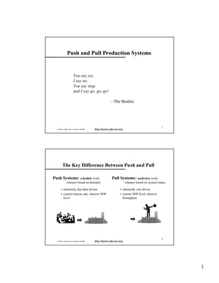
The Key Difference Between Push and Pull
Push Systems: schedule work

Pull Systems: authorize work

releases based on demand.
• inherently due-date driven
• control release rate, observe WIP
level


releases based on system status.
• inherently rate driven
• control WIP level, observe
throughput


2

1

Push vs. Pull Mechanics
PUSH

PULL

(Exogenous)
Schedule

(Endogenous)
Status

Production Process

Job

Job

Push systems are inherently
make-to-order.

Production Process

Pull systems are inherently
make-to-stock.
3


Pulling with Kanban
Outbound
stockpoint

Production
cards

Completed parts with cards
enter outbound stockpoint.

When stock is
removed, place
production card
in hold box.



Outbound
stockpoint

Production
card authorizes
start of work.

4

2

Push and Pull Line Schematics
Pure Push (MRP)

Stock
Point

Stock
Point

...

Pure Pull (Kanban)

Stock
Point

Stock
Point

...
…

Stock
Point

CONWIP

Authorization Signals

Stock
Point

...

Full Containers


5

Push/Pull Interface
Eliminate: entire portion of cycle time by building to stock.
Requirements:
• Level demand.
• Relatively few distinct parts.
• Relatively constant product mix.

Implementation:
• kanban
• late customization (postponement)



6

3

Example - Custom Taco Production Line
Push/Pull Interface
Pull

Push

Refrigerator

Cooking

Assembly

Packaging

Sales

Customer


7


Example - Quick Taco Production Line

Pull

Refrigerator

Cooking

Push/Pull Interface

Assembly

Packaging

Warming
Table



Push

Sales

Customer

8

4

The Magic of Pull
Pulling Everywhere?
You don’t never make nothin’ and send it no place. Somebody has to
come get it.

– Hall 1983
No! It’s the WIP Cap:
•Kanban – WIP cannot exceed number of cards
•“WIP explosions” are impossible


WIP


9

Advantages of Pull Systems
Low Unit Cost:

Good Customer Service:

• high throughput
• low inventory
• little rework

• short cycle times
• steady, predictable output stream

Flexibility:
High External Quality:
• high internal quality
• pressure for good quality
• promotion of good quality (e.g.,
defect detection)


• avoids committing jobs too early
• tolerates mix changes (within
limits)
• encourages floating capacity


10

5

Pull Benefits Achieved by WIP Cap
Reduces Manufacturing Costs:

Improves Quality:

• prevents WIP explosions
• reduces average WIP
• reduces engineering changes

Reduces Variability:

• pressure for higher quality
• improved defect detection
• improved communication

Maintains Flexibility:

• reduces cycle time variability
• pressure to reduce sources of
process time variability (e.g., long
repair times)
• promotes improved customer
service


• accommodates engineering
changes
• less direct congestion
• less reliance on forecasts
• air traffic control analogy

11


CONWIP
Assumptions:
1. Single routing
2. WIP measured in units

...

Mechanics: allow next job to enter line each time a job leaves (i.e., maintain a
WIP level of m jobs in the line at all times).

Modeling:
• MRP looks like an open queueing network
• CONWIP looks like a closed queueing network
• Kanban looks like a closed queueing network with blocking



12

6

CONWIP Controller
Work Backlog
PN
–—
–—
–—
–—
–—
–—
–—
–—
–—
–—
–—
–—
–—

Indicator Lights

Quant
–––––
–––––
–––––
–––––
–––––
–––––
–––––
–––––
–––––
–––––
–––––
–––––
–––––

LAN

R G

PC

PC

...
Workstations


13

CONWIP vs. Pure Push
Push/Pull Laws: A CONWIP system has the following advantages over an
equivalent pure push system:
1) Observability: WIP is observable; capacity is not.
2) Efficiency: A CONWIP system requires less WIP on average to attain a
given level of throughput.
3) Robustness: A profit function of the form
Profit = pTh - hWIP
is more sensitive to errors in TH than WIP.



14

7

CONWIP Efficiency Example
Equipment Data:
• 5 machines in tandem, all with capacity of one part/hr (u=TH·te=TH)
• exponential (moderate variability) process times

CONWIP System: looks like PWC, so
TH ( w) =

w
w
rb =
w + W0 − 1
w+ 4

Pure Push System: looks like series of M/M/1 queues, so
w(TH ) = 5

u
TH
=5
1− u
1 − TH

Comparison: WIP needed in CONWIP to match push throughput
w(

w
5( w /( w + 4))
5w
)=
=
w + 4 1 − ( w /( w + 4))
4

in this example, WIP
is always 25% higher
for same TH in push
than in CONWIP 15

CONWIP Robustness Example
Profit Function:

Profit = pTH − hw

 − hw
CONWIP: Profit(w) = p 
 w + 4

need to find “optimal”
WIP level

( )

need to find “optimal”
TH level (i.e., release
rate)

w

Push:

Profit(TH) = pTH − h

5 TH

1 − TH

Key Question: what happens when we don’t choose optimum
values (as we never will)?


16

8

CONWIP vs. Pure Push Comparisons
70

Optimum

CONWIP

60

Efficiency

50

Robustness

Profit

40
30

Push

20
10
0
0.00%
-10

20.00%

40.00%

60.00%

80.00%

100.00%

120.00%

140.00%

-20

Control as Percent of Opti mal


17

Modeling CONWIP with Mean-Value Analysis
Notation:
u j (w) = utilization of station j in CONWIP line with WIP level w
CT j (w) = cycle time at station j in CONWIP line with WIP level w
CT (w) =

n
j =1

CT j ( w) = cycle time of CONWIP line with WIP level w

TH (w) = throughput of CONWIP line with WIP level w
WIPj (w) = average WIP level at station j in CONWIP line with WIP level w

Basic Approach: Compute performance measures for increasing w
assuming job arriving to line “sees” other jobs distributed according
to average behavior with w-1 jobs.


18

9

Mean-Value Analysis Formulas
Starting with WIPj(0)=0 and TH(0)=0, compute for w=1,2,…
CT j ( w) =
CT ( w) =

t e2 ( j ) 2
[c e ( j ) − 1]TH ( w − 1) + [WIPj ( w − 1) + 1]t e ( j )
2
n

CT j ( w)
j =1

w
CT ( w)
WIPj ( w) = TH ( w)CT j ( w)
TH ( w) =


19


Computing Inputs for MVA
MEASURE:
Natural Process Time (hr)

STATION:
t0

1
0.090

2
0.090

3
0.094

4
0.090

5
0.090

Natural Process CV
Number of Machines
MTTF (hr)

2

c0
m
mf

0.500
1
200

0.500
1
200

0.500
1
200

0.500
1
200

0.500
1
200

MTTR (hr)
Availability
Effective Process Time (failures only)

mr
A
t e'

2
0.990
0.091

2
0.990
0.091

8
0.962
0.098

4
0.980
0.092

4
0.980
0.092

Eff Process CV (failures only)

ce '

2

0.936

0.936

6.795

2.209

2.209

Jobs Between Setups

Ns

100.000

100.000

100.000

100.000

100.000

Setup Time (hr)

ts

0.500

0.500

0.500

0.500

0.500

Setup Time CV

cs

1.000

1.000

1.000

1.000

1.000

Eff Process Time (failures+setups)

te

0.096

0.096

0.103

0.097

0.097

Eff Station Rate

re

10.428

10.428

9.731

10.331

10.331

Eff Process Time Var (failures+setups)

σe

2

0.013

0.013

0.070

0.024

0.024

2

1.382

1.382

6.621

2.517

2.517

Eff Process CV (failures+setups)

2

ce

rb
T0

0.488

W0

9.731
4.750


20

10

Output of MVA
TH

CT

w

Actual

Actual

1
2
3
4
5
6
7
8
9
10
11
12
13
14
15

2.049
2.928
3.644
4.185
4.629
5.000
5.317
5.592
5.834
6.049
6.241
6.414
6.572
6.715
6.846

0.488
0.683
0.823
0.956
1.080
1.200
1.317
1.431
1.543
1.653
1.763
1.871
1.978
2.085
2.191

CT1(w)

CT2(w)

0.096
0.118
0.134
0.149
0.163
0.176
0.189
0.202
0.214
0.226
0.237
0.249
0.260
0.271
0.283

0.096
0.118
0.134
0.149
0.163
0.176
0.189
0.202
0.214
0.226
0.237
0.249
0.260
0.271
0.283

CT3(w)
0.103
0.185
0.245
0.303
0.357
0.410
0.462
0.513
0.563
0.614
0.664
0.714
0.763
0.813
0.863

CT4(w)
0.097
0.131
0.155
0.177
0.198
0.219
0.238
0.257
0.276
0.294
0.312
0.330
0.347
0.364
0.381

CT5(w)
0.097
0.131
0.155
0.177
0.198
0.219
0.238
0.257
0.276
0.294
0.312
0.330
0.347
0.364
0.381
21



Using MVA to Evaluate Line Performance
12.000

10.000

8.000
Actual
Bes t Case

6.000

Wors t Case
PW C

4.000

2.000

0.000
0

5

10

15

20

25

30

35

WIP



22

11

Implementing Pull
Pull is Rigid:
• replenish stocks quickly (just in time)
• level mix, volume, sequence

JIT Practices
•
•
•
•

capacity buffers
setup reduction
flexible labor
facility layout



23

Capacity Buffers
Motivation: facilitate rapid replenishments with minimal WIP
Benefits:
• Protection against quota shortfalls
• Regular flow allows matching against customer demands
• Can be more economical in long run than WIP buffers in push systems

Techniques:
• Planned underutilization (e.g., use u = 75% in aggregate planning)
• Two shifting: 4 – 8 – 4 – 8
• Schedule dummy jobs to allow quick response to hot jobs



24

12

Setup Reduction
Motivation: Small lot sequences not feasible with large setups.
Internal vs. External Setups:
• External – performed while machine is still running
• Internal – performed while machine is down

Approach:
1. Separate the internal setup from the external setup
2. Convert as much as possible of the internal setup to the external setup
3. Eliminate the adjustment process
4. Abolish the setup itself (e.g., uniform product design, combined
production, parallel machines)


25


Flexible Labor
Cross-Trained Workers:
• float where needed
• appreciate line-wide perspective
• provide more heads per problem area

Shared Tasks:
• can be done by adjacent stations
• reduces variability in tasks, and hence line stoppages/quality problems
work can float to
workers, or workers
can float to work…



26

13

Cellular Layout
Advantages:
• Better flow control
• Improved material handling (smaller transfer batches)
• Ease of communication (e.g., for floating labor)

Challenges:
• May require duplicate equipment
• Product to cell assignment
Inbound Stock


Outbound Stock

27


Focused Factories
Pareto Analysis:
• Small percentage of sku’s represent large percentage of volume
• Large percentage of sku’s represent little volume but much complexity

Dedicated Lines:
Drill

Drill

Paint

Mill

Drill

Paint

Weld

Grind

Lathe

Assembly

Mill

Mill

Grind

Drill

Grind

Paint

Lathe

Assembly

Stores

Saw

Warehouse

Job Shop Environment:
• for low runners
• many setups
• poorer performance, but only
on smaller portion of business
• may need to use push

Lathe

Saw

Warehouse

Saw

Stores

• for families of high runners
• few setups
• can use pull effectively

Mill
Drill



28

14

Push/Pull Takeaways
Magic of Pull: the WIP cap
Logistical Benefits of Pull:
• observability
• efficiency
• robustness (this is the key one)

Overcoming Rigidity of Pull:
•
•
•
•
•

capacity buffers
setup reduction
flexible labor
facility layout
many others (postponement, push/pull hybrids, etc.… )



29

15

Push and pull production system

Recommandé

Recommandé

Contenu connexe

Tendances

Tendances (20)

En vedette

En vedette (7)

Similaire à Push and pull production system

Similaire à Push and pull production system (11)

Dernier

Dernier (20)

Push and pull production system