SlideShare une entreprise Scribd logo
1  sur  158
Télécharger pour lire hors ligne
1
UNIT 1
1.1 Introduction:
1. The Python Programming Language:
1 The programming language you will be learning is Python. Python is an example of a
high-level language; other high-level languages you might have heard of are C++,
PHP, and Java.
2 As you might infer from the name high-level language, there are also low-level
languages, sometimes referred to as machine languages or assembly languages.
Loosely speaking, computers can only execute programs written in low-level
languages. Thus, programs written in a high-level language have to be processed
before they can run. This extra processing takes some time, which is a small
disadvantage of high-level languages.
3 But the advantages are enormous. First, it is much easier to program in a high-level
language. Programs written in a high-level language take less time to write, theyare
shorter and easier to read, and they are more likely to be correct. Second, high-level
languages are portable, meaning that they can run on different kinds of computers
with few or no modifications. Low-level programs can run on only one kind of
computer and have to be rewritten to run on another.
4 Due to these advantages, almost all programs are written in high-level languages.
Low-level languages are used only for a few specialized applications.
5 Two kinds of applications process high-level languages into low-level languages:
interpreters and compilers. An interpreter reads a high-level program and executes
it, meaning that it does what the program says. It processes the program a little at a
time, alternately reading lines and performing computations.
6
7 A compiler reads the program and translates it into a low-level program, which can
then be run.
8 In this case, the high-level program is called the source code, and the translated
program is called the object code or the executable. Once a program is compiled,
you can execute it repeatedly without further translation.
9
10 Many modern languages use both processes. They are first compiled into a lower
level language, called byte code, and then interpreted by a program called a virtual
machine. Python uses both processes, but because of the way programmers interact
with it, it is usually considered an interpreted language.
11 There are two ways to use the Python interpreter: shell mode and script mode. In shell
mode, you type Python statements into the Python shell and the interpreter
SOURCE
CODE
COMPILER EXECUTOR OUTPUTOBJECT
CODE
OUTPUTSOURCE
CODE
INTERPRETER
2
immediately prints the result.
12 In this course, we will be using an IDE (Integrated Development Environment)called
IDLE. When you first start IDLE it will open an interpreter window.1
13 The first few lines identify the version of Python being used as well as a few other
messages; you can safely ignore the lines about the firewall. Next there is a line
identifying the version of IDLE. The last line starts with >>>, which is the Python
prompt. The interpreter uses the prompt to indicate that it is ready for instructions.
14 If we type print 1 + 1 the interpreter will reply 2 and give us another prompt.2
15 >>> print 1 + 1
16 2
17 >>>
18 Alternatively, you can write a program in a file and use the interpreter to execute the
contents of the file. Such a file is called a script. For example, we used the text editor
in IDLE (but we could have used any text editor) to create a file named
firstprogram.py with the following contents:
19 print 1 + 1
20 By convention, files that contain Python programs have names that end with .py. To
execute the program we have to invoke the interpreter and tell it the name of the
script:
21 $ python firstprogram.py
22 2
This example shows Python being run from a terminal (with $ representing the Unix prompt).
In other development environments, the details of executing programs may differ. IDLE
simplifies the whole process by presenting interpreter windows and a text editor within the
same application. You can run a script in IDLE by either choosing Run → Run Module or
pressing F5. Most programs are more interesting than this one. The examples in this book use
both the Python interpreter and scripts. You will be able to tell which is intended since shell
mode examples (i.e. entering lines directly into the interpreter) will always start with the
Python prompt, >>>. Working in shell mode is convenient for testing short bits of code
because you get immediate feedback. Think of it as scratch paper used to help you work out
problems. Anything longer than a few lines should be put into a script so it can be saved for
future use.
2. History of Python:
Python was developed by Guido van Rossum in the late eighties and early nineties at the
National Research Institute for Mathematics and Computer Science in the Netherlands.
1 You can also run the python interpreter by just entering the command python in a terminal. To exit from the interpreter type exit() and hit
return, or press Ctrl-D on a new line.
2 The print statement is one of the changes between Python 2.x and Python 3.x. In Python 3.x, print is a function and not a
3
• Python is derived from many other languages, including ABC, Modula-3, C, C++,
Algol-68, SmallTalk, and Unix shell and other scripting languages.
• Python is copyrighted. Like Perl, Python source code is now available under the GNU
General Public License (GPL).
• Python is now maintained by a core development team at the institute, although Guido
van Rossum still holds a vital role in directing its progress.
• Python 1.0 was released in November 1994. In 2000, Python 2.0 was released. Python
2.7.11 is the latest edition of Python 2.
• Meanwhile, Python 3.0 was released in 2008. Python 3 is not backward compatible
with Python 2. The emphasis in Python 3 had been on the removal of duplicate
programming constructs and modules so that "There should be one -- and preferably
only one -- obvious way to do it." Python 3.5.1 is the latest version of Python 3.
3. Features of python:
Python's features include-
• Easy-to-learn: Python has few keywords, simple structure, and a clearly defined
syntax. This allows a student to pick up the language quickly.
• Easy-to-read: Python code is more clearly defined and visible to the eyes.
• Easy-to-maintain: Python's source code is fairly easy-to-maintain.
• A broad standard library: Python's bulk of the library is very portable and
crossplatform compatible on UNIX, Windows, and Macintosh.
• Interactive Mode: Python has support for an interactive mode, which allows
interactive testing and debugging of snippets of code.
• Portable: Python can run on a wide variety of hardware platforms and has the same
interface on all platforms.
• Extendable: You can add low-level modules to the Python interpreter. These modules
enable programmers to add to or customize their tools to be more efficient.
• Databases: Python provides interfaces to all major commercial databases.
• GUI Programming: Python supports GUI applications that can be created and ported
4
to many system calls, libraries and windows systems, such as Windows MFC,
Macintosh, and the X Window system of Unix.
• Scalable: Python provides a better structure and support for large programs than shell
scripting.
Apart from the above-mentioned features, Python has a big list of good features. A few are
listed below-
• It supports functional and structured programming methods as well as OOP.
• It can be used as a scripting language or can be compiled to byte-code for building
large applications.
• It provides very high-level dynamic data types and supports dynamic type checking.
• It supports automatic garbage collection.
• It can be easily integrated with C, C++, COM, ActiveX, CORBA, and Java.
4. Installing Python:
5
Windows platform
Binaries of latest version of Python 3 (Python 3.5.1) are available on this download page
The following different installation options are available.
• Windows x86-64 embeddable zip file  Windows x86-64 executable installer 
Windows x86-64 web-based installer
• Windows x86 embeddable zip file Windows x86 executable installer
• Windows x86 web-based installer
Note:In order to install Python 3.5.1, minimum OS requirements are Windows 7 with SP1. For
versions 3.0 to 3.4.x, Windows XP is acceptable.
Linux platform
Different flavors of Linux use different package managers for installation of new packages.
On Ubuntu Linux, Python 3 is installed using the following command from the terminal.
Installation from source
Mac OS
Download Mac OS installers from this URL:https://www.python.org/downloads/mac-osx/
• Mac OS X 64-bit/32-bit installer : python-3.5.1-macosx10.6.pkg
• Mac OS X 32-bit i386/PPC installer : python-3.5.1-macosx10.5.pkg
Double click this package file and follow the wizard instructions to install.
The most up-to-date and current source code, binaries, documentation, news, etc., is available
on the official website of Python:
Download Gzipped source tarball from Python's download
URL: https://www.python.org/ftp/python/3.5.1/Python-
3.5.1.tgz Extract the tarball tar xvfz Python-3.5.1.tgz Configure
and Install:
cd Python-3.5.1
./configure --prefix=/opt/python3.5.1 make
sudo make install
$sudo apt-get install python3-minimal
6
Python Official Website : http://www.python.org/
You can download Python documentation from the following site. The documentation is
available in HTML, PDF and PostScript formats.
Python Documentation Website : www.python.org/doc/
Setting up PATH
Programs and other executable files can be in many directories. Hence, the operating systems
provide a search path that lists the directories that it searches for executables.
The important features are-
• The path is stored in an environment variable, which is a named string maintained by
the operating system. This variable contains information available to the command
shell and other programs.
• The path variable is named as PATH in Unix or Path in Windows (Unix is
casesensitive; Windows is not).
• In Mac OS, the installer handles the path details. To invoke the Python interpreter from
any particular directory, you must add the Python directory to your path.
Setting Path at Unix/Linux
To add the Python directory to the path for a particular session in Unix-
• In the csh shell: type setenv PATH "$PATH:/usr/local/bin/python3" and pressEnter.
• In the bash shell (Linux): type export PATH="$PATH:/usr/local/bin/python3" and
press Enter.
• In the sh or ksh shell: type PATH="$PATH:/usr/local/bin/python3" and pressEnter.
Note: /usr/local/bin/python3 is the path of the Python directory.
Setting Path at Windows
To add the Python directory to the path for a particular session in Windows-
At the command prompt : type path
%path%;C:Python and press Enter.
7
Note: C:Python is the path of the Python directory.
Python Environment Variables
Here are important environment variables, which are recognized by Python-
Variable Description
PYTHONPATH
It has a role similar to PATH. This variable tells the Python
interpreter where to locate the module files imported into a program.
It should include the Python source library directory and the
directories containing Python source code. PYTHONPATH is
sometimes, preset by the Python installer.
PYTHONSTARTU
P
It contains the path of an initialization file containing Python source
code. It is executed every time you start the interpreter. It is named
as .pythonrc.py in Unix and it contains commands that load utilities
or modify PYTHONPATH.
PYTHONCASEOK It is used in Windows to instruct Python to find the first
caseinsensitive match in an import statement. Set this variable to
any value to activate it.
PYTHONHOME It is an alternative module search path. It is usually embedded in the
PYTHONSTARTUP or PYTHONPATH directories to make
switching module libraries easy.
5. Running Python program:
There are three different ways to start Python-
(1) Interactive Interpreter
You can start Python from Unix, DOS, or any other system that provides you a commandline
interpreter or shell window.
Enter python the command line.
8
Start coding right away in the interactive interpreter.
Here is the list of all the available command line options-
Option Description
-d provide debug output
-O generate optimized bytecode (resulting in .pyo files)
-S do not run import site to look for Python paths on startup
-v verbose output (detailed trace on import statements)
-X disable class-based built-in exceptions (just use strings); obsolete starting with
version 1.6
-c cmd run Python script sent in as cmd string
file run Python script from given file
(2) Script from the Command-line
A Python script can be executed at the command line by invoking the interpreter on your
application, as shown in the following example.
Note: Be sure the file permission mode allows execution.
(3) Integrated Development Environment
$python
python%
C:>python
# Unix/Linux or
# Unix/Linux or
# Windows/DOS
$python script.py
python% script.py
C:>python script.py
# Unix/Linux or
# Unix/Linux or
# Windows/DOS
9
You can run Python from a Graphical User Interface (GUI) environment as well, if you have a
GUI application on your system that supports Python.
• Unix: IDLE is the very first Unix IDE for Python.
• Windows: PythonWin is the first Windows interface for Python and is an IDE with a
GUI.
• Macintosh: The Macintosh version of Python along with the IDLE IDE is available
from the main website, downloadable as either MacBinary or BinHex'd files.
If you are not able to set up the environment properly, then you can take the help of your
system admin. Make sure the Python environment is properly set up and working perfectly
fine.
6. Debugging:
Programming is a complex process, and because it is done by human beings, programs
often contain errors. For whimsical reasons, programming errors are called bugs and the
process of tracking them down and correcting them is called debugging.
Three kinds of errors can occur in a program: syntax errors, runtime errors, and semantic
errors. It is useful to distinguish between them in order to track them down more quickly.
Syntax errors
Python can only execute a program if the program is syntactically correct; otherwise,
the process fails and returns an error message. Syntax refers to the structure of a
program and the rules about that structure. For example, in English, a sentence must
begin with a capital letter and end with a period. this sentence contains a syntax
error. So does this one
For most readers, a few syntax errors are not a significant problem, which is why we
can read the poetry of e. e. cummings without spewing error messages. Python is not
so forgiving. If there is a single syntax error anywhere in your program, Python will
print an error message and quit, and you will not be able to run your program.
During the first few weeks of your programming career, you will probably spend a
lot of time tracking down syntax errors. As you gain experience, though, you will
make fewer syntax errors and find them faster.
Runtime errors
The second type of error is a runtime error, so called because the error does not
appear until you run the program. These errors are also called exceptions because
they usually indicate that something exceptional (and bad) has happened. Runtime
errors are rare in the simple programs you will see in the first few chapters, so it
might be a while before you encounter one.
10
Semantic errors
The third type of error is the semantic error. If there is a semantic error in your
program, it will run successfully, in the sense that the computer will not generate
any error messages, but it will not do the right thing. It will do something else.
Specifically, it will do what you told it to do.
The problem is that the program you wrote is not the program you wanted to write.
The meaning of the program (its semantics) is wrong. Identifying semantic errors
can be tricky because it requires you to work backward by looking at the output of
the program and trying to figure out what it is doing.
One of the most important skills you will acquire is debugging. Although it can be
frustrating, debugging is one of the most intellectually rich, challenging, and interesting
parts of programming.
In some ways, debugging is like detective work. You are confronted with clues, and you
have to infer the processes and events that led to the results you see.
Debugging is usually a trial and error process. Once you have an idea what is going
wrong, you modify your program and try again. If your hypothesis was correct, then you
can predict the result of the modification, and you take a step closer to a working
program. If your hypothesis was wrong, you have to come up with a new one. As
Sherlock Holmes pointed out, “When you have eliminated the impossible, whatever
remains, however improbable, must be the truth.” (A. Conan Doyle, The Sign of Four )
For some people, programming and debugging are the same thing. That is, programming
is the process of gradually debugging a program until it does what you want. The idea is
that you should start with a program that does something and make small modifications,
debugging them as you go, so that you always have a working program.
For example, Linux is an operating system that contains thousands of lines of code, but it
started out as a simple program Linus Torvalds used to explore the Intel 80386 chip.
According to Larry Greenfield, one of Linus’s earlier projects was a program that would
switch between printing AAAA and BBBB. This later evolved into Linux (The Linux Users’
Guide Beta Version 1).
7. Formal and Natural Languages:
Natural languages are the languages that people speak, such as English, Spanish, and
French. They were not designed by people (although people try to impose some order on
them); they evolved naturally.
Formal languages are languages that are designed by people for specific applications.
For example, the notation that mathematicians use is a formal language that is particularly
good at denoting relationships among numbers and symbols. Chemists use a formal
11
language to represent the chemical structure of molecules. And most importantly:
Programming languages are formal languages that have been designed to express
computations.
Formal languages tend to have strict rules about syntax. For example, 3+3=6 is a
syntactically correct mathematical statement, but 3=+6$ is not. H2O is a syntactically
correct chemical name, but 2Zz is not. Syntax rules come in two flavors, pertaining to
tokens and structure. Tokens are the basic elements of the language, such as words,
numbers, and chemical elements. One of the problems with 3=+6$ is that $ is not a legal
token in mathematics (at least as far as we know). Similarly, 2Zz is not legal because
there is no element with the abbreviation Zz. The second type of syntax rule pertains to
the structure of a statement— that is, the way the tokens are arranged. The statement
3=+6$ is structurally illegal because you can’t place a plus sign immediately after an
equal sign. Similarly, molecular formulas have to have subscripts after the element name,
not before.
When you read a sentence in English or a statement in a formal language, you have to
figure out what the structure of the sentence is (although in a natural language you do this
subconsciously). This process is called parsing. For example, when you hear the
sentence, “The brown dog barked”, you understand that the brown dog is the subject and
barked is the verb. Once you have parsed a sentence, you can figure out what it means, or
the semantics of the sentence. Assuming that you know what a dog is and what it means
to bark, you will understand the general implication of this sentence.
Although formal and natural languages have many features in common—tokens,
structure, syntax, and semantics—there are many differences:
ambiguity: Natural languages are full of ambiguity, which people deal with by using
contextual clues and other information. Formal languages are designed to be nearly
or completely unambiguous, which means that any statement has exactly one
meaning, regardless of context.
redundancy: In order to make up for ambiguity and reduce misunderstandings, natural
languages employ lots of redundancy. As a result, they are often verbose. Formal
languages are less redundant and more concise.
literalness: Natural languages are full of idiom and metaphor. If someone says, “The
penny dropped”, there is probably no penny and nothing dropped. Formal languages
mean exactly what they say.
People who grow up speaking a natural language—everyone—often have a hard time
adjusting to formal languages. In some ways, the difference between formal and natural
language is like the difference between poetry and prose, but more so:
Poetry: Words are used for their sounds as well as for their meaning, and the whole poem
together creates an effect or emotional response. Ambiguity is not only common but
often deliberate.
Prose: The literal meaning of words is more important, and the structure contributes
12
more meaning. Prose is more amenable to analysis than poetry but still often
ambiguous.
Programs: The meaning of a computer program is unambiguous and literal, and can be
understood entirely by analysis of the tokens and structure.
Here are some suggestions for reading programs (and other formal languages). First,
remember that formal languages are much more dense than natural languages, so it takes
longer to read them. Also, the structure is very important, so it is usually not a good idea to
read from top to bottom, left to right. Instead, learn to parse the program in your head,
identifying the tokens and interpreting the structure. Finally, the details matter. Little things
like spelling errors and bad punctuation, which you can get away with in natural languages,
can make a big difference in a formal language.
8. The Difference Between Brackets, Braces, and Parentheses:
Braces are used for different purposes. If you just want a list to contain some elements and
organize them by index numbers (starting from 0), just use the [] and add elements as
necessary. {} are special in that you can give custom id's to values like a = {"John":
14}. Now, instead of making a list with ages and remembering whose age is where, you can
just access John's age by a["John"].
The [] is called a list and {} is called a dictionary (in Python). Dictionaries are basically a
convenient form of list which allow you to access data in a much easier way.
However, there is a catch to dictionaries. Many times, the data that you put in the dictionary
doesn't stay in the same order as before. Hence, when you go through each value one by one, it
won't be in the order you expect. There is a special dictionary to get around this, but you have
to add this line from collections import OrderedDict and replace {} with OrderedDict(). But, I
don't think you will need to worry about that for now.
1.2 Variables and Expressions:
1. Values and Types:
A value is one of the fundamental things—like a letter or a number—that a program
manipulates. The values we have seen so far are 2 (the result when we added 1 + 1),
and “Hello, World!”. These values belong to different types: 2 is an integer, and
“Hello, World!” is a string. You (and the interpreter) can identify strings because
they are enclosed in quotation marks.
The print statement also works for integers.
>>> print(4)
4
If you are not sure what type a value has, the interpreter can tell you.
>>> type("Hello, World!")
13
Strings belong to the type str and integers belong to the type int. Less obviously,
numbers with a decimal point belong to a type called float, because these numbers
are represented in a format called floating-point.
What about values like “17” and “3.2”? They look like numbers, but they are in
quotation marks like strings.
<class ’str’>
They’re strings. Strings in Python can be enclosed in either single quotes (’) or
double quotes (”):
Double quoted strings can contain single quotes inside them, as in "What’s your
name?", and single quoted strings can have double quotes inside them, as in ’The cat
said "Meow!"’.
When you type a large integer, you might be tempted to use commas between groups of three
digits, as in 1,000,000.
2. Variables:
One of the most powerful features of a programming language is the ability to
manipulate variables. A variable is a name that refers to a value. The assignment
statement creates new variables and assigns them values:
<class ’str’>
>>> type(17)
< class ’int’>
>>> type(3.2)
<class ’float’>
>>> type("17")
<class ’str’>
>>> type("3.2")
>>> type(’This is a string.’)
<class ’str’>
>>> type("And so is this.")
<class ’str’>
>>> message = "What’s your name?"
>>> n = 17
>>> pi = 3.14159
14
This example makes three assignments. The first assigns the string "What’s your
name?" to a new variable named message. The second assigns the integer 17 to n, and
the third assigns the floating-point number 3.14159 to pi. The assignment operator,
=, should not be confused with an equals sign (even though it uses the same
character). Assignment operators link a name, on the left hand side of the operator,
with a value, on the right hand side. This is why you will get an error if you enter:
A common way to represent variables on paper is to write the name with an arrow
pointing to the variable’s value. This kind of figure is called a state diagram because
it shows what state each of the variables is in (think of it as the variable’s state of
mind). This diagram shows the result of the assignment statements:
messag
e n pi
"What’s your name?"
17
3.14159
The print statement also works with variables.
In each case the result is the value of the variable. Variables also have types; again,
we can ask the interpreter what they are.
The type of a variable is the type (or kind) of value it refers to.
>>> 17 = n
>>>print (message)
What’s your name?
>>> print (n)
17
>>> print (pi)
3.14159
>>> type(message)
<class ’str’>
>>> type(n)
< class ’int’>
>>> type(pi)
< class ’float’>
15
3. Variable names and keywords:
Programmers generally choose names for their variables that are meaningful—they
document what the variable is used for. Variable names can be arbitrarily long. They
can contain both letters and numbers, but they have to begin with a letter. Although it
is legal to use uppercase letters, by convention we don’t. If you do, remember that
case matters. Bruce and bruce are different variables. The underscore character ( ) can
appear in a name. It is often used in names with multiple words, such as myname or
priceofteainchina. If you give a variable an illegal name, you get a syntax error:
76trombones is illegal because it does not begin with a letter. more$ is illegal because
it contains an illegal character, the dollar sign. But what’s wrong with class? It turns
out that class is one of the Python keywords. Keywords define the language’s rules
and structure, and they cannot be used as variable names. Python has thirty-one
keywords:
and del from not while
as elif global or with
assert else if pass yield
break except import print
class exec in raise
continue finally is return
def for lambda try
4. Type conversion:
Sometimes, you may need to perform conversions between the built-in types. To convert
between types, you simply use the type-name as a function.
There are several built-in functions to perform conversion from one data type to another.
>>> 76trombones = "big parade"
SyntaxError: invalid syntax
>>> more$ = 1000000
SyntaxError: invalid syntax
>>> class = "COMP150"
SyntaxError: invalid syntax
16
These functions return a new object representing the converted value.
Function Description
int(x [,base])
Converts x to an integer. The base specifies the base if x is a string.
float(x) Converts x to a floating-point number.
complex(real
[,imag])
Creates a complex number.
str(x) Converts object x to a string representation.
repr(x) Converts object x to an expression string.
eval(str) Evaluates a string and returns an object.
tuple(s) Converts s to a tuple.
list(s) Converts s to a list.
set(s) Converts s to a set.
dict(d) Creates a dictionary. d must be a sequence of (key,value) tuples.
frozenset(s) Converts s to a frozen set.
chr(x) Converts an integer to a character.
unichr(x) Converts an integer to a Unicode character.
17
ord(x) Converts a single character to its integer value.
hex(x) Converts an integer to a hexadecimal string.
oct(x) Converts an integer to an octal string.
5. Operators and Operands:
Operators are special symbols that represent computations like addition and
multiplication. The values the operator uses are called operands. The following are
all legal Python expressions whose meaning is more or less clear:
The symbols +, -, *, /, have the usual mathematical meanings. The symbol, **, is the
exponentiation operator. The statement, 5 ** 2, means 5 to the power of 2, or 5
squared in this case. Python also uses parentheses for grouping, so we can force
operations to be done in a certain order just like we can in mathematics.
When a variable name appears in the place of an operand, it is replaced with its value
before the operation is performed. Addition, subtraction, multiplication, and
exponentiation all do what you expect, but you might be surprised by division. The
following operation has an unexpected result:
The value of minute is 59, and 59 divided by 60 is 0.98333, not 0. The reason for the
discrepancy is that Python is performing integer division3
. When both of the
operands are integers, the result must also be an integer, and by convention, integer
division always rounds down, even in cases like this where the next integer is very
close. A possible solution to this problem is to calculate a percentage rather than a
fraction:
20 + 32 hour - 1 hour * 60 + minute minute / 60
5 ** 2
(5 + 9) * (15 - 7)
>>> minute = 59
>>> minute / 60
0 .9833333333333333
>>> minute * 100 / 60
18
Operators are special symbols that represent computations like addition and
multiplication. The values the operator uses are called operands. The following are
all legal Python expressions whose meaning is more or less clear:
The symbols +, -, *, /, have the usual mathematical meanings. The symbol, **, is the
exponentiation operator. The statement, 5 ** 2, means 5 to the power of 2, or 5
squared in this case. Python also uses parentheses for grouping, so we can force
operations to be done in a certain order just like we can in mathematics.
When a variable name appears in the place of an operand, it is replaced with its value
before the operation is performed. Addition, subtraction, multiplication, and
exponentiation all do what you expect, but you might be surprised by division. The
following operation has an unexpected result:
The value of minute is 59, and 59 divided by 60 is 0.98333, not 0. The reason for the
discrepancy is that Python is performing integer division4
. When both of the
operands are integers, the result must also be an integer, and by convention, integer
division always rounds down, even in cases like this where the next integer is very
close. A possible solution to this problem is to calculate a percentage rather than a
fraction:
Again the result is rounded down, but at least now the answer is approximately correct.
Another alternative is to use floating-point division.
6. Expressions:
An expression is a combination of values, variables, and operators. If you type an
expression on the command line, the interpreter evaluates it and displays the result:
20 + 32 hour - 1 hour * 60 + minute minute / 60
5 ** 2
(5 + 9) * (15 - 7)
>>> minute = 59
>>> minute / 60
0 .9833333333333333
>>> minute * 100 / 60
98.33333333333333
>>> 1 + 1
2
19
The evaluation of an expression produces a value, which is why expressions can
appear on the right hand side of assignment statements. A value all by itself is a
simple expression, and so is a variable.
Confusingly, evaluating an expression is not quite the same thing as printing a value.
>>> message = "What’s your name?"
>>> message
"What’s your name?"
>>> print(message)
What’s your name?
When the Python shell displays the value of an expression, it uses the same format
you would use to enter a value. In the case of strings, that means that it includes the
quotation marks. But the print statement prints the value of the expression, which in
this case is the contents of the string. In a script, an expression all by itself is a legal
statement, but it doesn’t do anything. The script
17
3.2
"Hello, World!"
1 + 1
produces no output at all. How would you change the script to display the values of
these four expressions?
7. Interactive Mode and Script Mode:
Interactive Mode Programming
Invoking the interpreter without passing a script file as a parameter brings up the following
prompt-
>>> 17
17
>>> x
2
20
$ python
Python 3.3.2 (default, Dec 10 2013, 11:35:01)
[GCC 4.6.3] on Linux
Type "help", "copyright", "credits", or "license" for more information. >>>
On Windows:
Python 3.4.3 (v3.4.3:9b73f1c3e601, Feb 24 2015, 22:43:06) [MSC v.1600 32 bit (Intel)] on
win32
Type "copyright", "credits" or "license()" for more information.
>>>
Type the following text at the Python prompt and press Enter-
If you are running the older version of Python (Python 2.x), use of parenthesis as inprint
function is optional. This produces the following result-
Script Mode Programming
Invoking the interpreter with a script parameter begins execution of the script and continues
until the script is finished. When the script is finished, the interpreter is no longer active.
Let us write a simple Python program in a script. Python files have the extension.py. Type the
following source code in a test.py file-
We assume that you have the Python interpreter set in PATH variable. Now, try to run this
program as follows-
On Linux
This produces the following result-
On Windows
This produces the following result-
>>> print ("Hello, Python!")
Hello, Python!
print ("Hello, Python!")
$ python test.py
Hello, Python!
C:Python34>Python test.py
21
Let us try another way to execute a Python script in Linux. Here is the modified test.py
file-
We assume that you have Python interpreter available in the /usr/bin directory. Now, try to run
this program as follows-
This produces the following result-
Order of Operations:
When more than one operator appears in an expression, the order of evaluation
depends on the rules of precedence. Python follows the same precedence rules for its
mathematical operators that mathematics does. The acronym PEMDAS is a useful
way to remember the order of operations:
1. Parentheses have the highest precedence and can be used to force an expression
to evaluate in the order you want. Since expressions in parentheses are evaluated
first, 2*(3-1) is 4, and (1+1)**(5-2) is 8. You can also use parentheses to make
an expression easier to read, as in (minute*100)/60, even though it doesn’t
change the result.
2. Exponentiation has the next highest precedence, so 2**1+1 is 3 and not 4, and
3*1**3 is 3 and not 27.
3. Multiplication and Division have the same precedence, which is higher than
Addition and Subtraction, which also have the same precedence. So 2*3-1 yields
5 rather than 4, and 2/3-1 is -1, not 1 (remember that in integer division, 2/3=0).
Operators with the same precedence are evaluated from left to right. So in the
expression minute*100/60, the multiplication happens first, yielding 5900/60, which
in turn yields 98. If the operations had been evaluated from right to left, the result
would have been 59*1, which is 59, which is wrong. Similarly, in evaluating 17-4-3,
Hello, Python!
#!/usr/bin/python3 print
("Hello, Python!")
$ chmod +x test.py # This is to make file executable
$./test.py
Hello, Python!
22
17-4 is evaluated first.
If in doubt, use parentheses.
1.3 Conditional Statements:
1. IF statement:
The IF statement is similar to that of other languages. The if statement contains a logical
expression using which the data is compared and a decision is made based on the result of the
comparison.
Syntax
If the boolean expression evaluates to TRUE, then the block of statement(s) inside the if
statement is executed. In Python, statements in a block are uniformly indented after the :
symbol. If boolean expression evaluates to FALSE, then the first set of code after the end of
block is executed.
if expression: statement(s)
23
Flow Diagram
nested if statements You can use one if or else if statement inside another if
or else if statement(s).
Example
When the above code is executed, it produces the following result −
num = 3
if num > 0:
print(num, "is a positive number.")
print("This is always printed.")
num = -1 if
num > 0:
print(num, "is
a positive number.")
print("This is
also always
printed.")
24
3 is a positive number.
This is always printed.
In the above example, num > 0 is the test expression.
The body of if is executed only if this evaluates to True.
When variable num is equal to 3, test expression is true and body inside body of if is executed.
If variable num is equal to -1, test expression is false and body inside body of if is skipped.
The print() statement falls outside of the if block (unindented). Hence, it is executed regardless
of the test expression.
2. IF ELSE Statements
An else statement can be combined with an if statement. An else statement contains a block of
code that executes if the conditional expression in the if statement resolves to 0 or a FALSE
value.
The else statement is an optional statement and there could be at the most only one else
statement following if.
Syntax
The syntax of the if...else statement is-
if expression:
statement(s) else:
statement(s)
Flow Diagram
25
Positive or Zero
Example
# Program checks if the number is positive or negative
# And displays an appropriate message
num = 3
# Try these two variations as well.
# num = -5
# num = 0
if num >= 0:
print("Positive or Zero")
else:
print("Negative number")
In the above example, when num is equal to 3, the test expression is true and body of if is
executed and body of else is skipped.
If num is equal to -5, the test expression is false and body of else is executed and body
26
of if is skipped.
3. Nested IF -ELSE Statements
There may be a situation when you want to check for another condition after a condition
resolves to true. In such a situation, you can use the nested if construct.
In a nested if construct, you can have an if...elif...else construct inside another if...elif...else
construct.
Syntax
The syntax of the nested if...elif...else construct may be-
if expression1:
statement(s)
if expression2:
statement(s)
elif expression3:
statement(s)
else
statement(s)
elif expression4:
statement(s)
else:
statement(s)
27
Example
When the above code is executed, it produces the following result-
# !/usr/bin/python3
# In this program, we input a number
# check if the number is positive or
# negative or zero and display
# an appropriate message
# This time we use nested if
num = float(input("Enter a number: "))
if num >= 0:
if num == 0:
print("Zero")
else:
print("Positive number")
else:
print("Negative number")
num=int(input("enter number"))
Output 1
Enter a number: 5
Positive number
Output 2
Enter a number: -1
Negative number
Output 3
Enter a number: 0
Zero Divisible by 3 and 2
enter number5
28
not Divisible by 2 not divisible by 3
1.4 Looping:
1. For:
The for loop in Python is used to iterate over a sequence (list, tuple, string) or other iterable
objects. Iterating over a sequence is called traversal.
Syntax of for Loop
for val in sequence:
Body of for
Here, val is the variable that takes the value of the item inside the sequence on each iteration.
Loop continues until we reach the last item in the sequence. The body of for loop is separated
from the rest of the code using indentation.
Flowchart of for Loop
29
Example: Python for Loop
# Program to find the sum of all numbers stored in
a list
# List of numbers
numbers = [6, 5, 3, 8, 4, 2, 5, 4, 11]
# variable to store the sum
sum = 0
# iterate over the list
for val in numbers:
30
sum = sum+val
# Output: The sum is 48
print("The sum is", sum)
when you run the program, the output will be:
The sum is 48
2. While Loop
The while loop in Python is used to iterate over a block of code as long as the test expression
(condition) is true.
We generally use this loop when we don't know beforehand, the number of times to iterate.
Syntax of while Loop in Python
while test_expression:
Body of while
In while loop, test expression is checked first. The body of the loop is entered only if
the test_expression evaluates to True. After one iteration, the test expression is checked again.
This process continues until the test_expression evaluates to False.
In Python, the body of the while loop is determined through indentation.
Body starts with indentation and the first unindented line marks the end.
Python interprets any non-zero value as True. None and 0 are interpreted as False.
Flowchart of while Loop
31
Example: Python while Loop
# Program to add natural
# numbers upto
# sum = 1+2+3+...+n
# To take input from the user,
# n = int(input("Enter n: "))
n = 10
# initialize sum and counter
32
When you run the program, the output will be:
In the above program, the test expression will be True as long as our counter variable i is less
than or equal to n (10 in our program).
We need to increase the value of counter variable in the body of the loop. This is very
important (and mostly forgotten). Failing to do so will result in an infinite loop (never ending
loop).
Finally the result is displayed.
3. Nested loops:
Python programming language allows to use one loop inside another loop. Following section
shows few examples to illustrate the concept.
sum = 0
i = 1
while i <= n:
sum = sum + i
i = i+1 # update counter
# print the sum
print("The sum is", sum)
Enter n: 10
The sum is 55
33
Python Nested if Example
# In this program, we input a number
# check if the number is positive or
# negative or zero and display
# an appropriate message
# This time we use nested if
num = float(input("Enter a number: "))
if num >= 0:
if num == 0:
print("Zero")
else:
print("Positive number")
else:
print("Negative number")
Output 1
Enter a number: 5
Positive number
Output 2
Enter a number: -1
Negative number
Output 3
Enter a number: 0
Zero
1.5 Control statements:
1. Terminating loops:
The break statement terminates the loop containing it. Control of the program flows to the
statement immediately after the body of the loop.
34
If break statement is inside a nested loop (loop inside another loop), break will terminate the
innermost loop.
Syntax of break
Flowchart of break
break
35
Example: Python break
Output
In this program, we iterate through the "string" sequence. We check if the letter is "i", upon
# Use of break statement inside loop
for val in "string":
if val == "i":
break
print(val)
print("The end")
s
t
r
The end
36
which we break from the loop. Hence, we see in our output that all the letters up till "i" gets
printed. After that, the loop terminates.
2. Skipping specific conditions:
The continue statement is used to skip the rest of the code inside a loop for the current iteration
only. Loop does not terminate but continues on with the next iteration.
Syntax of Continue
continue
Flowchart of continue
The working of continue statement in for and while loop is shown below.
37
Example: Python continue
Output
# Program to show the use of continue statement inside loops
for val in "string":
if val == "i":
continue
print(val)
print("The end")
s
t
38
This program is same as the above example except the break statement has been replaced with
continue.
We continue with the loop, if the string is "i", not executing the rest of the block. Hence, we
see in our output that all the letters except "i" gets printed.
r
n
g
The end
39
40
UNIT 2
FUNCTIONS :
2.1 Composing Expressions
So far, we have looked at the elements of a program—variables, expressions, and
statements —in isolation, without talking about how to combine them. One of the
most useful features of programming languages is their ability to take small building
blocks and compose them. For example, we know how to add numbers and we know
how to print; it turns out we can do both at the same time:
In reality, the addition has to happen before the printing, so the actions aren’t
actually happening at the same time. The point is that any expression involving
numbers, strings, and variables can follow print:
You can also put arbitrary expressions on the right-hand side of an assignment
statement:
This ability may not seem impressive now, but you will see other examples where
the composition makes it possible to express complex computations neatly and
concisely.
Warning: There are limits on where you can use certain expressions. For example,
left-hand side of an assignment statement has to be a variable name, not an
expression. So, the following is illegal:
3.2 Function calls
Many common tasks come up time and time again when programming. Instead of
requiring you to constantly reinvent the wheel, Python has a number of built-in
features which you can use. Including so much ready to use code is sometimes
>>> print(17 + 3)
20
>>> hour = 21
>>> minute = 1
>>> print("Number of minutes since midnight: ",hour * 60 + minute)
Number of minutes since midnight: 1261
>>> percentage = (minute * 100) / 60
>>> percentage
1.6666666666666667
>>> print(percentage)
1.6666666666666667
>>> minute+1 = hour
File "<stdin>", line 1
SyntaxError: can't assign to operator
41
referred to as a ’batteries included’ philosophy. Python comes with just under fifty
(of which we’ll be only using about a dozen) and the simplest way to use this
prewritten code is via function calls.
The syntax of a function call is simply
FUNCTION NAME(ARGUMENTS)
Not all functions take an argument, and some take more than one (in which case the
arguments are separated by commas).
You have already seen an example of a function call:
>>> type("Hello,World")
<class 'str'>
>>> type(17)
<class 'int'>
The name of the function is type, and it displays the type of a value or variable. The
value or variable, which is called the argument of the function, has to be enclosed in
parentheses. It is common to say that a function “takes” an argument and “returns” a
result. The result is called the return value.
We can assign the return value to a variable:
Another useful function is len. It takes a Python sequence as an argument. The only
Python sequence we have met so far is a string. A string is a sequence of characters.
For a string argument, len returns the number of characters the string contains.
The len function can only be used on sequences. Trying to use it on a number, for
example, results in an error.
2.3 Type Conversion Functions :
Each Python type comes with a built-in function that attempts to convert values of
another type into that type. The int(ARGUMENT) function, for example, takes any
value and converts it to an integer, if possible, or complains otherwise:
>>> result = type(17)
>>> print(result)
<class 'int'>
>>> my_str = "Hello world"
>>> len(my_str)
11
>>> len(3)
Traceback (most recent call last):
File "<stdin>", line 1, in <module>
TypeError: object of type 'int' has no len()
>>> int("32")
42
The int function can also convert floating-point values to integers, but note that it
truncates the fractional part:
The float(ARGUMENT) function converts integers and strings to floating-point
numbers:
>>> float(32)
32.0
>>> float("3.14159")
3.14159
>>> float(1)
1.0
It may seem odd that Python distinguishes the integer value 1 from the floating-point
value 1.0. They may represent the same number, but they belong to different types as
they are represented differently inside the computer.
The str(ARGUMENT) function converts any argument to type string:
The str(ARGUMENT) function will work with any value and convert it into a string.
Note: True is a predefined value in Python; true is not.
2.4 Math Functions :
Python includes following functions that perform mathematical calculations.
32
>>> int("Hello")
Traceback (most recent call last):
File "<stdin>", line 1, in <module>
ValueError: invalid literal for int() with base 10: 'Hello'
>>> int(-2.3)
-2
>>> int(3.99999)
3
>>> int("42")
42
>>> int(1.0)
1
>>> str(32)
'32'
>>> str(3.14149)
'3.14149'
>>> str(True)
'True'
>>> str(true)
Traceback (most recent call last): File
"<stdin>", line 1, in <module>
NameError: name 'true' is not defined
43
Function Returns ( description )
abs(x) The absolute value of x: the (positive) distance between x and zero.
ceil(x) The ceiling of x: the smallest integer not less than x
cmp(x, y) -1 if x < y, 0 if x == y, or 1 if x > y
exp(x) The exponential of x: ex
fabs(x) The absolute value of x.
floor(x) The floor of x: the largest integer not greater than x
log(x) The natural logarithm of x, for x> 0
log10(x) The base-10 logarithm of x for x> 0.
max(x1, x2,...) The largest of its arguments: the value closest to positive infinity
min(x1, x2,...) The smallest of its arguments: the value closest to negative infinity
modf(x)
The fractional and integer parts of x in a two-item tuple. Both
parts have the same sign as x. The integer part is returned as a
float.
pow(x, y) The value of x**y.
round(x [,n])
x rounded to n digits from the decimal point. Python rounds away
from zero as a tie-breaker: round(0.5) is 1.0 and round(-0.5) is -1.0.
Number abs() Method :
Description: The abs() method returns the absolute value of x i.e. the positive distance
between x and zero.
Syntax : Following is the syntax for abs() method-
abs(x)
Parameters :
x - This is a numeric expression.
Return : This method returns the absolute value of x.
The following example shows the usage of the abs() method.
print ("abs(-45) : ", abs(-45))
print ("abs(100.12) : ", abs(100.12))
44
When we run the above program, it produces the following result-
Number ceil() Method :
Description: The ceil() method returns the ceiling value of x i.e. the smallest integer
not less than x.
Syntax: Following is the syntax for the ceil() method
import math
math.ceil( x )
Note: This function is not accessible directly, so we need to import math module and
then we need to call this function using the math static object.
Parameters
x - This is a numeric expression.
Return Value
This method returns the smallest integer not less than x.
Example
The following example shows the usage of the ceil() method.
When we run the above program, it produces the following result
Number exp() Method
Description
The exp() method returns exponential of x: ex.
Syntax
Following is the syntax for the exp() method
Note: This function is not accessible directly. Therefore, we need to import the math
module and then we need to call this function using the math static object.
Parameters
X - This is a numeric expression.
Return Value
This method returns exponential of x: ex.
abs(-45): 45
abs(100.12) : 100.12
import math # This will import math module
print ("math.ceil(-45.17) : ", math.ceil(-45.17))
print ("math.ceil(100.12) : ", math.ceil(100.12))
print ("math.ceil(100.72) : ", math.ceil(100.72))
print ("math.ceil(math.pi) : ", math.ceil(math.pi))
math.ceil(-45.17) : -45
math.ceil(100.12) : 101
math.ceil(100.72) : 101
math.ceil(math.pi) : 4
import math
math.exp( x )
45
Example
The following example shows the usage of exp() method.
When we run the above program, it produces the following result
Number fabs() Method
Description
The fabs() method returns the absolute value of x. Although similar to the abs()
function, there are differences between the two functions. They are-
• abs() is a built in function whereas fabs() is defined in math module.
• fabs() function works only on float and integer whereas abs() works with
complex number also.
Syntax
Following is the syntax for the fabs() method
Note: This function is not accessible directly, so we need to import the math module
and
then we need to call this function using the math static object.
Parameters
x - This is a numeric value.
Return Value
This method returns the absolute value of x.
Example
The following example shows the usage of the fabs() method.
When we run the above program, it produces following result
import math # This will import math module
print ("math.exp(-45.17) : ", math.exp(-45.17))
print ("math.exp(100.12) : ", math.exp(100.12))
print ("math.exp(100.72) : ", math.exp(100.72))
print ("math.exp(math.pi) : ", math.exp(math.pi))
math.exp(-45.17) : 2.4150062132629406e-20
math.exp(100.12) : 3.0308436140742566e+43
math.exp(100.72) : 5.522557130248187e+43
math.exp(math.pi) : 23.140692632779267
import math
math.fabs( x )
import math # This will import math module
print ("math.fabs(-45.17) : ", math.fabs(-45.17))
print ("math.fabs(100.12) : ", math.fabs(100.12))
print ("math.fabs(100.72) : ", math.fabs(100.72))
print ("math.fabs(math.pi) : ", math.fabs(math.pi))
math.fabs(-45.17) : 45.17
46
Number floor() Method
Description
The floor() method returns the floor of x i.e. the largest integer not greater than x.
Syntax
Following is the syntax for the floor() method
Note: This function is not accessible directly, so we need to import the math module
and then we need to call this function using the math static object.
Parameters
x - This is a numeric expression.
Return Value
This method returns the largest integer not greater than x.
The following example shows the usage of the floor() method.
When we run the above program, it produces the following result
Number log() Method
Description
The log() method returns the natural logarithm of x, for x > 0.
Syntax
Following is the syntax for the log() method
Note: This function is not accessible directly, so we need to import the math module
and then we need to call this function using the math static object.
Parameters
math.fabs(100.12) : 100.12
math.fabs(100.72) : 100.72
math.fabs(math.pi) : 3.141592653589793
import math
math.floor( x )
import math # This will import math module
print ("math.floor(-45.17) : ", math.floor(-45.17))
print ("math.floor(100.12) : ", math.floor(100.12))
print ("math.floor(100.72) : ", math.floor(100.72))
print ("math.floor(math.pi) : ", math.floor(math.pi))
math.floor(-45.17) : -46
math.floor(100.12) : 100
math.floor(100.72) : 100
math.floor(math.pi) : 3
import math
math.log( x )
47
x - This is a numeric expression.
Return Value
This method returns natural logarithm of x, for x > 0.
Example
The following example shows the usage of the log() method.
When we run the above program, it produces the following result
Number log10() Method
Description
The log10() method returns base-10 logarithm of x for x > 0.
Syntax
Following is the syntax for log10() method
Note: This function is not accessible directly, so we need to import the math module
and then we need to call this function using the math static object.
Parameters
x - This is a numeric expression.
Return Value
This method returns the base-10 logarithm of x for x > 0.
Example
The following example shows the usage of the log10() method.
import math # This will import math module
print ("math.log10(100.12) : ", math.log10(100.12))
print ("math.log10(100.72) : ", math.log10(100.72))
print ("math.log10(119) : ", math.log10(119))
print ("math.log10(math.pi) : ", math.log10(math.pi))
When we run the above program, it produces the following result
Number max() Method
Description
import math # This will import math module
print ("math.log(100.12) : ", math.log(100.12))
print ("math.log(100.72) : ", math.log(100.72))
print ("math.log(math.pi) : ", math.log(math.pi))
math.log(100.12) : 4.6063694665635735
math.log(100.72) : 4.612344389736092
math.log(math.pi) : 1.1447298858494002
import math
math.log10( x )
math.log10(100.12) : 2.0005208409361854
math.log10(100.72) : 2.003115717099806
math.log10(119) : 2.0755469613925306
math.log10(math.pi) : 0.49714987269413385
48
The max() method returns the largest of its arguments i.e. the value closest to positive
infinity.
Syntax
Following is the syntax for max() method
Parameters
• x - This is a numeric expression.
• y - This is also a numeric expression.
• z - This is also a numeric expression.
Return Value
This method returns the largest of its arguments.
Example
The following example shows the usage of the max() method.
When we run the above program, it produces the following result
Number min() Method
Description
The method min() returns the smallest of its arguments i.e. the value closest to
negative
infinity.
Syntax
Following is the syntax for the min() method
Parameters
• x - This is a numeric expression.
• y - This is also a numeric expression.
• z - This is also a numeric expression.
Return Value
This method returns the smallest of its arguments.
Example
The following example shows the usage of the min() method.
max(x, y, z, .... )
print ("max(80, 100, 1000) : ", max(80, 100, 1000))
print ("max(-20, 100, 400) : ", max(-20, 100, 400))
print ("max(-80, -20, -10) : ", max(-80, -20, -10))
print ("max(0, 100, -400) : ", max(0, 100, -400))
max(
80, 100, 1000) : 1000
max(-20, 100, 400) : 400
max(-80, -20, -10) : -10
max(0, 100, -400) : 100
min(x, y, z, .... )
print ("min(80, 100, 1000) : ", min(80, 100, 1000))
49
When we run the above program, it produces the following result
Number modf() Method
Description
The modf() method returns the fractional and integer parts of x in a two-item tuple.
Both parts have the same sign as x. The integer part is returned as a float.
Syntax
Following is the syntax for the modf() method
Note: This function is not accessible directly, so we need to import the math module
and then we need to call this function using the math static object.
Parameters
x - This is a numeric expression.
Return Value
This method returns the fractional and integer parts of x in a two-item tuple. Both the
parts have the same sign as x. The integer part is returned as a float.
Example
The following example shows the usage of the modf() method.
When we run the above program, it produces the following result
Number pow() Method
Return Value
This method returns the value of xy.
Example
The following example shows the usage of the pow() method.
print ("min(-20, 100, 400) : ", min(-20, 100, 400))
print ("min(-80, -20, -10) : ", min(-80, -20, -10))
print ("min(0, 100, -400) : ", min(0, 100, -400))
min(80, 100, 1000) : 80
min(-20, 100, 400) : -20
min(-80, -20, -10) : -80
min(0, 100, -400) : -400
import math
math.modf( x )
import math # This will import math module
print ("math.modf(100.12) : ", math.modf(100.12))
print ("math.modf(100.72) : ", math.modf(100.72))
print ("math.modf(119) : ", math.modf(119))
print ("math.modf(math.pi) : ", math.modf(math.pi))
math.modf(100.12) : (0.12000000000000455, 100.0)
math.modf(100.72) : (0.7199999999999989, 100.0)
math.modf(119) : (0.0, 119.0)
math.modf(math.pi) : (0.14159265358979312, 3.0)
50
When we run the above program, it produces the following result
Number round() Method
Description
round() is a built-in function in Python. It returns x rounded to n digits from the
decimal point.
Syntax
Following is the syntax for the round() method
Parameters
• x - This is a numeric expression.
• n - Represents number of digits from decimal point up to which x is to be
rounded.
Default is 0.
Return Value
This method returns x rounded to n digits from the decimal point.
Example
The following example shows the usage of round() method
When we run the above program, it produces the following result
Number sqrt() Method
Description
import math # This will import math module
print ("math.pow(100, 2) : ", math.pow(100, 2))
print ("math.pow(100, -2) : ", math.pow(100, -2))
print ("math.pow(2, 4) : ", math.pow(2, 4))
print ("math.pow(3, 0) : ", math.pow(3, 0))
math.
pow(100, 2) : 10000.0
math.pow(100, -2) : 0.0001
math.pow(2, 4) : 16.0
math.pow(3, 0) : 1.0
round(x [, n] )
print ("round(70.23456) : ", round(70.23456))
print ("round(56.659,1) : ", round(56.659,1))
print ("round(80.264, 2) : ", round(80.264, 2))
print ("round(100.000056, 3) : ", round(100.000056, 3))
print ("round(-100.000056, 3) : ", round(-100.000056, 3))
round(70.23456) : 70
round(56.659,1) : 56.7
round(80.264, 2) : 80.26
round(100.000056, 3) : 100.0
round(-100.000056, 3) : -100.0
51
The sqrt() method returns the square root of x for x > 0.
Syntax
Following is the syntax for sqrt() method
Note: This function is not accessible directly, so we need to import the math module
and then we need to call this function using the math static object.
Parameters
x - This is a numeric expression.
Return Value
This method returns square root of x for x > 0.
Example
The following example shows the usage of sqrt() method.
When we run the above program, it produces the following result
2.5 Function Composition :
Just as with mathematical functions, Python functions can be composed, meaning that
you use the result of one function as the input to another.
In the first example, abs(-7) evaluates to 7, which then becomes the argument to
print twice. In the second example we have two levels of composition, since abs(-
11) is first evaluated to 11 before max(3, 1, 11, 7) is evaluated to 11 and (11)
print_twice then displays the result.
We can also use a variable as an argument:
import math
math.sqrt( x )
import math # This will import math module
print ("math.sqrt(100) : ", math.sqrt(100))
print ("math.sqrt(7) : ", math.sqrt(7))
print ("math.sqrt(math.pi) : ", math.sqrt(math.pi))
math.sqrt(100) : 10.0
math.sqrt(7) : 2.6457513110645907
math.sqrt(math.pi) : 1.7724538509055159
>>> def print_twice(some_variable_name):
... print(some_variable_name, some_variable_name)
...
>>> print_twice(abs(-7))
7 7
>>> print_twice(max(3,1,abs(-11),7))
11 11
52
Notice something very important here. The name of the variable we pass as an
argument (saying) has nothing to do with the name of the parameter
(some_variable_name). It doesn’t matter what the argument is called; here in
print_twice, we call everybody some_variable_name.
2.5 Adding New Functions
A new function can be created in python using keyword def followed by the function
name and arguments in parathesis and statements to be executed in function
Example:
def requiredArg (str,num):
statements
2.6 Function definitions and use
As well as the built-in functions provided by Python you can define your own
functions. In the context of programming, a function is a named sequence of
statements that performs a desired operation. This operation is specified in a function
definition. In Python, the syntax for a function definition is:
The ’list of parameters’ is where the arguments supplied to the function end up.
You will see more of this later.
You can make up any names you want for the functions you create, except that you
can’t use a name that is a Python keyword. The list of parameters specifies what
information, if any, you have to provide in order to use the new function.
There can be any number of statements inside the function, but they have to be you.
indented from the def. In the examples in this book, we will use the standard
indentation of four spaces3. IDLE automatically indents compound statements for
Function definitions are the first of several compound statements we will see, all
of which have the same pattern:
1. A header, which begins with a keyword and ends with a colon.
2. A body consisting of one or more Python statements, each indented the same
amount – 4 spaces is the Python standard – from the header.
In a function definition, the keyword in the header is def, which is followed by the
list name of the function and a list of parameters enclosed in parentheses. The
parameter may be empty, or it may contain any number of parameters. In either
case, the parentheses are required. The first couple of functions we are going to no
write have parameters, so the syntax looks like this:
>>> saying = "Eric,the half a bee."
>>> print_twice(saying)
Eric,the half a bee. Eric,the half a bee.
def NAME( LIST OF PARAMETERS ):
STATEMENTS
53
This function is named new_line. The empty parentheses indicate that it has no
which parameters (that is it takes no arguments). Its body contains only a single
statement, outputs a newline character. (That’s what happens when you use a print
command without any arguments.)
Defining a new function does not make the function run. To do that we need a by a
function call. Function calls contain the name of the function to be executed
followed list of values, called arguments, which are assigned to the parameters in
the function definition. Our first examples have an empty parameter list, so the do
function calls not take any arguments. Notice, however, that the parentheses are
required in the function call :
... print("First Line.")
... new_line()
... print("Second Line")
The output of the function is :
First Line.
Second Line
The extra space between the two lines is a result of the new line() function call.
What if we wanted more space between the lines? We could call the same function
repeatedly:
... print("First Line.")
... new_line()
... new_line()
... new_line()
... print("Second Line")
Or we could write a new function named three lines that prints three new lines:
This function contains three statements, all of which are indented by four spaces.
Since the next statement is not indented, Python knows that it is not part of the
function. You should notice a few things about this program:
• You can call the same procedure repeatedly. In fact, it is quite common and
useful to do so.
• You can have one function call another function; in this case three lines calls
new_line.
>>> def new_line() :
... print()
>>> def three_lines() :
... new_line()
... new_line()
... new_line()
... print("First Line.")
... three_lines()
... print("Second Line.")
54
So far, it may not be clear why it is worth the trouble to create all of these new
functions. Actually, there are a lot of reasons, but this example demonstrates two:
1. Creating a new function gives you an opportunity to name a group of
statements. Functions can simplify a program by hiding a complex computation
behind a single command and by using English words in place of arcane code.
2. Creating a new function can make a program smaller by eliminating repetitive
code. For example, a short way to print nine consecutive new lines is to call
three lines three times.
Pulling together the code fragments from the previous section into a script named
functions.py, the whole program looks like this:
This program contains two function definitions: new_line and three_lines. Function
to definitions get executed just like other statements, but the effect is to create the
new function. The statements inside the function do not get executed until the is
called, and the function definition generates no output. As you might expect, you
have create a function before you can execute it. In other words, the function
definition has to be executed before the first time it is called.
2.7 Flow of Execution
In order to ensure that a function is defined before its first use, you have to know
the order in which statements are executed, which is called the flow of execution.
Execution always begins at the first statement of the program. Statements are
executed one at a time, in order from top to bottom. Function definitions do not
alter the flow of execution of the program, but remember that statements inside the
function are not executed until the function is called. Although it is not common,
you can define one function inside another. In this case, the inner definition isn’t
executed until the outer function is called.
Function calls are like a detour in the flow of execution. Instead of going to the next
statement, the flow jumps to the first line of the called function, executes all the
statements there, and then comes back to pick up where it left off. That sounds
simple enough, until you remember that one function can call another. While in the
middle of one function, the program might have to execute the statements in another
function. But while executing that new function, the program might have to execute
def new_line() :
print()
def three_lines() :
new_line()
new_line()
new_line()
print("First Line.")
three_lines()
print("Second Line.")
55
yet another function! Fortunately, Python is adept at keeping track of where it is, so
each time a function completes, the program picks up where it left off in the
function that called it. When it gets to the end of the program, it terminates.
It is usually not helpful to read a program from top to bottom. In python programs
the top part of a file is almost always used for function definitions and it is not
necessary to read those until you want to understand what a particular function
does. The bottom part of a python file is often called the main program. This part
can be recognised because it is often not indented. It is easier to understand a the
program by following flow of execution starting at the beginning of the main
program.
2.8 Parameters and Arguments
Most functions require arguments. Arguments are values that are input to the function
and these contain the data that the function works on. For example, if you want to find
the absolute value of a number (the distance of a number from zero) you have to
indicate what the number is. Python has a built-in function for computing the absolute
value:
In this example, the arguments to the abs function are 5 and -5.
Some functions take more than one argument. For example the built-in function pow
takes two arguments, the base and the exponent. Inside the function, the values that are
passed get assigned to variables called parameters.
The first argument is raised to the power of the second argument.
round(), not surprisingly, rounds a number and returns the floating point value first is
rounded to n-digits digits after the decimal point. It takes one or two arguments. The
number to be rounded and the second (optional) value is the number of digits to round
to. If the second number is not supplied it is assumed to be zero.
>>> abs(5)
5
>>> abs(-5)
5
>>> pow(2,3)
8
>>> pow(3,2)
9
>>> round(1.23456789)
1
>>> round(1.5)
2
>>> round(1.23456789,2)
1.23
56
Another built-in function that takes more than one argument is max.
The function max can be sent any number of arguments, separated by commas, and
will return the maximum value sent. The arguments can be either simple values or
expressions. In the last example, 503 is returned, since it is larger than 33, 125, and 1.
Here is an example of a user-defined function that has a parameter:
This function takes a single argument and assigns it to the parameter named will be) is
some_variable_name. The value of the parameter (at this point we have no idea what it
printed twice, followed by a newline. The name some_variable_name was chosen to
suggest that the name you give a parameter is up to you,but in general, you want to
choose something more descriptive than some_variable_name.
In a function call, the value of the argument is assigned to the corresponding parameter
in the function definition. In effect, it is as if some_variable_name = "Spam" is
executed when print_twice("Spam") is called; some_variable_name = 5 is executed
when print_twice(5) is called; and some_variable_name = 3.14159 is executed when
print_twice(3.14159) is called. Any type of argument that can be printed can be sent to
print_twice. In the first function call, the argument is a string. In the second, it’s an
integer. In the third, it’s a float.
As with built-in functions, we can use an expression as an argument for print twice:
"Spam"*4 is first evaluated to ’SpamSpamSpamSpam’, which is then passed as an
argument to print_twice.
2.9 Variable and Parameters are Local
>>> def print_joined_twice(part1, part2) :
... joined = part1 + part2
... print_twice(joined)
This function takes two arguments, concatenates them and stores the result in a local
variable joined. It then calls print twice with joined as the argument. print twice prints
the value of the argument, twice. We can call the function with two strings:
>>> round(1.23456789,3)
1.235
>>> max(7,11)
11
>>> max(1,4,17,2,12)
17
>>> max(3*11, 5**3, 512-9, 1024**0)
503
>>> def print_twice(some_variable_name):
... print(some_variable_name, some_variable_name)
>>> print_twice("Spam"*4)
SpamSpamSpamSpam SpamSpamSpamSpam
57
When print joined twice terminates, the variable joined is destroyed. If we try to print
it, we get an error:
When you create a local variable inside a function, it only exists inside that function,
and you cannot use it outside. Parameters are also local. For example, outside the
function print_twice, there is no such thing as phrase. If you try to use it, Python will
complain. Similarly, part1 and part2 do not exist outside print_joined_twice.
2.10 Stack Diagrams
To keep track of which variables can be used where, it is sometimes useful to draw a
stack diagram. Like state diagrams, stack diagrams show the value of each variable, but
they also show the function to which each variable belongs. Each function is
represented by a frame. A frame is a box with the name of a function beside it and the
parameters and variables of the function inside it. The stack diagram for the previous
example looks like this:
print_twice
print_joined_twice
_main_
The order of the stack shows the flow of execution. print_twice was called by
print_joined_twice, and print_joined_twice was called by _main_ , which is a special
name for the topmost function. When you create a variable outside of any function, it
belongs to _main_ . Each parameter refers to the same value as its corresponding
argument. So, part1 has the same value as line1, part2 has the same value as line2, and
phrase has the same value as joined. If an error occurs during a function call, Python
prints the name of the function, and the name of the function that called it, and the
name of the function that called that, all the way back to the top most function. To see
how this works, we create a Python script named stacktrace.py that looks like this:
>>> line1 = "Happy birthday,"
>>> line2 = "to you."
>>> print_joined_twice(line1, line2)
Happy birthday,to you. Happy birthday,to you.
>>> print(joined)
Traceback (most recent call last):
File "<stdin>", line 1, in <module>
NameError: name 'joined' is not defined
phrase "Happy birthday, to you."
part1
part2
joined
"Happy birthday, "
"to you."
"Happy birthday, to you."
line1
line2
"Happy birthday, "
"to you."
58
We’ve added the statement, print joined inside the print twice function, but joined is
not defined there. Running this script will produce an error message like this:
This list of functions is called a traceback. It tells you what program file the error
occurred in, and what line, and what functions were executing at the time. It also shows
the line of code that caused the error. Notice the similarity between the traceback and
the stack diagram. It’s not a coincidence. In fact, another common name for a traceback
is a stack trace.
2.11 Fruitful functions and Void functions
2.11.1 The return statement
The return statement allows you to terminate the execution of a function before
you reach the end. One reason to use it is if you detect an error condition:
The function print square root has a parameter named x. The first thing it does is check
whether x is less than 0, in which case it displays an error message and then uses return
to exit the function. The flow of execution immediately returns to the caller, and the
remaining lines of the function are not executed.
def print_twice(phrase):
print(phrase, phrase)
print(joined)
def print_joined_twice(part1, part2):
joined = part1 + part2
print_twice(joined)
line1 = "Happy birthday, "
line2 = "to you."
print_joined_twice(line1, line2)
Traceback (most recent call last):
File "C:/Python34/example.py", line 11, in <module>
print_joined_twice(line1, line2)
File "C:/Python34/example.py", line 7, in print_joined_twice
print_twice(joined)
File "C:/Python34/example.py", line 3, in print_twice
print(joined)
NameError: name 'joined' is not defined
def print_square_root(x):
if x < 0:
print("Warning: cannot take square root of a negative number.")
return
result = x**0.5
print("The square root of x is", result)
59
2.11.2 Return values
The built-in functions we have used, such as abs, pow, round and max, have produced
results. Calling each of these functions generates a value, which we usually assign to a
variable or use as part of an expression.
So far, none of the functions we have written has returned a value, they have printed
values. In this lecture, we are going to write functions that return values, which we will
call fruitful functions, for want of a better name. The first example is area_of_circle,
which returns the area of a circle with the given radius:
We have seen the return statement before, but in a fruitful function the return statement
includes a return value. This statement means: Return immediately from this function
and use the following expression as a return value. The expression provided can be
arbitrarily complicated, so we could have written this function more concisely:
On the other hand, temporary variables like area often make debugging easier.
Sometimes it is useful to have multiple return statements, one in each branch of a
conditional. For instance, we have already seen the built-in abs, now we see how to
write our own:
Since these return statements are in an alternative conditional, only one will be
executed. As soon as one is executed, the function terminates without executing any
subsequent statements. Another way to write the above function is to leave out the else
and just follow if the condition by the second return statement.
biggest = max(3, 7, 2, 5)
x = abs(3 - 11) + 10
def area_of_circle(radius):
if radius < 0:
print("Warning: radius must be non-negative")
return
area = 3.14159 * radius**2
return area
def area_of_circle(radius):
if radius < 0:
print("Warning: radius must be non-negative")
return
return 3.14159 * radius**2
def absolute_value(x):
if x < 0:
return -x
else:
return x
def absolute_value(x):
if x < 0:
return -x
60
Think about this version and convince yourself it works the same as the first one. Code
that appears any place the flow of execution can never reach, is called dead code. In a
fruitful function, it is a good idea to ensure that every possible path through the
program hits a return statement. The following version of absolute value fails to do
this:
This version is not correct because if x happens to be 0, neither condition is true, and
the function ends without hitting a return statement. In this case, the return value is a
special value called None:
None is the unique value of a type called the NoneType:
All Python functions return None whenever they do not return another value. So the
earlier functions we wrote that didn’t have a return statement were actually returning
values, we just never checked.
2.11.3 Program Development
At this point, you should be able to look at complete functions and tell what they do.
Also, while completing the laboratory exercises given so far, you will have written
some small functions. As you write larger functions, you might start to have more
difficulty, especially with runtime and semantic errors. To deal with increasingly
complex programs, we are going to suggest a technique called incremental
development. The goal of incremental development is to avoid long debugging
sessions by adding and testing only a small amount of code at a time.
return x
def absolute_value(x):
if x < 0:
return -x
elif x > 0:
return x
>>> print(absolute_value(0))
None
>>> type(None)
<class 'NoneType'>
>>> def print_hello() :
print("hello")
>>> return_value = print_hello()
hello
>>> type(return_value)
<class 'NoneType'>
61
As an example, suppose you want to find the distance between two points, given by the
coordinates (x1, y1) and (x2, y2). By the Pythagorean theorem, the distance is:
distance =�(𝑥𝑥𝑥𝑥2 − 𝑥𝑥𝑥𝑥1)2 + (𝑦𝑦𝑦𝑦2 − 𝑦𝑦𝑦𝑦1)2
The first step is to consider what a distance function should look like in Python. In
other words, what are the inputs (parameters) and what is the output (return value)? In
this case, the two points are the inputs, which we can represent using four parameters.
The return value is the distance, which is a floating-point value. Already we can write
an outline of the function:
Obviously, this version of the function doesn’t compute distances; it always returns
zero. But it is syntactically correct, and it will run, which means that we can test it
before we make it more complicated. To test the new function, we call it with sample
values:
We chose these values so that the horizontal distance equals 3 and the vertical distance
equals 4; that way, the result is 5 (the hypotenuse of a 3-4-5 triangle). When testing a
function, it is useful to know the right answer. At this point we have confirmed that the
function is syntactically correct, and we can start adding lines of code. After each
incremental change, we test the function again. If an error occurs at any point, we
know where it must be—in the last line we added.
A logical first step in the computation is to find the differences x2 − x1 and y2 − y1.
We will store those values in temporary variables named dx and dy and print them.
If the function is working, the outputs should be 3 and 4. If so, we know that the
function is getting the right parameters and performing the first computation correctly.
If not, there are only a few lines to check.
Next we compute the sum of squares of dx and dy:
def distance(x1, y1, x2, y2):
return 0.0
>>> distance(1,2,4,6)
0.0
def distance(x1, y1, x2, y2):
dx = x2 - x1
dy = y2 - y1
print("dx is", dx)
print("dy is", dy)
return 0.0
def distance(x1, y1, x2, y2):
dx = x2 - x1
dy = y2 - y1
dsquared = dx**2 + dy**2
print("dsquared is: ", dsquared)
62
Notice that we removed the print statements we wrote in the previous step. Code like
that is called scaffolding because it is helpful for building the program but is not part of
the final product. Again, we would run the program at this stage and check the output
(which should be 25). Finally, using the fractional exponent 0.5 to find the square root,
we compute and return the result:
If that works correctly, you are done. Otherwise, you might want to print the value of
result before the return statement. When you start out, you should add only a line or
two of code at a time. As you gain more experience, you might find yourself writing
and debugging bigger chunks. Either way, the incremental development process can
save you a lot of debugging time. The key aspects of the process are:
1. Start with a working program and make small incremental changes. At any
point, if there is an error, you will know exactly where it is.
2. Use temporary variables to hold intermediate values so you can output and
check them.
3. Once the program is working, you might want to remove some of the
scaffolding or consolidate multiple statements into compound expressions, but
only if it does not make the program difficult to read.
2.11.4 Composition
As you should expect by now, you can call one function from within another. This
ability is called composition. As an example, we’ll write a function that takes two
points, the center of the circle and a point on the perimeter, and computes the area of
the circle. Assume that the center point is stored in the variables xc and yc, and the
perimeter point is in xp and yp. The first step is to find the radius of the circle, which is
the distance between the two points. Fortunately, we’ve just written a function,
distance, that does just that, so now all we have to do is use it:
The second step is to find the area of a circle with that radius and return it. Again we
will use one of our earlier functions:
Wrapping that up in a function, we get:
return 0.0
def distance(x1, y1, x2, y2):
dx = x2 - x1
dy = y2 - y1
dsquared = dx**2 + dy**2
result = dsquared**0.5
return result
radius = distance(xc, yc, xp, yp)
result = area_of_circle(radius)
def area_of_circle_two_points(xc, yc, xp, yp):
radius = distance(xc, yc, xp, yp)
result = area_of_circle(radius)
63
We called this function area of circle two points to distinguish it from the
area_of_circle function defined earlier. There can only be one function with a given
name within a given module. The temporary variables radius and result are useful for
development and debugging, but once the program is working, we can make it more
concise by composing the function calls:
2.11.5 Boolean functions
Functions can return boolean values, which is often convenient for hiding complicated
tests inside functions. For example:
The name of this function is is divisible. It is common to give boolean functions names
that sound like yes/no questions. is_divisible returns either True or False to indicate
whether the x is or is not divisible by y. We can make the function more concise by
taking advantage of the fact that the condition of the if statement is itself a boolean
expression. We can return it directly, avoiding the if statement altogether:
This session shows the new function in action:
Boolean functions are often used in conditional statements:
It might be tempting to write something like:
return result
def area_of_circle_two_points(xc, yc, xp, yp):
return area_of_circle(distance(xc, yc, xp, yp))
>>> def is_divisible(x, y):
if x % y == 0:
return True
else:
return False
def is_divisible(x, y):
return x % y == 0
>>> is_divisible(6,4)
False
>>> is_divisible(6,3)
True
if is_divisible(x, y):
print("x is divisible by y")
else:
print("x is not divisible by y")
if is_divisible(x, y) == True:
print("x is divisible by y")
64
But the extra comparison is unnecessary.
2.11.6 Void Functions
Void functions are functions, like ‘print_twice’ (that we defined earlier), that perform
an action (either display something on the screen or perform some other action).
However, they do not return a value.
For instance, we defined the function ‘print_twice’. The function is meant to perform
the action of printing twice the parameter ‘bruce’.
In interactive mode:Python will display the result of a void function if and only if we
call a function in interactive mode.
In script mode:When we call a fruitful function all by itself in script mode, the return
value is lost forever if we do not store or display the result.
For instance:
It is important to note that although Python displayed the value of result earlier, the
result displayed:
Bing
Bing
is lost forever since we did not store it anywhere.
In order to transmit this idea Python created the notion of ‘None’. It is a special value
that has its own type.
2.12 Importing with from
We can use functions in modules in three different ways:
 Import a module object in Python:If you import math, you get a module object
named math. The module object contains constants like pi and functions like sin
and exp.
else:
print("x is not divisible by y")
>>> def print_twice(some_variable):
… print(some_variable)
…
>>> result = print_twice(‘Bing’)
Bing
Bing
>>> print result
None
>>> print(type(None))
<class 'NoneType'>
65
 Import an object from a module in Python
Now you can access pi directly, without dot notation.
 Import all objects from a module in Python
The advantage of importing everything from the math module is that your code can be
more concise. The disadvantage is that there might be conflicts between names defined
in different modules, or between a name from a module and one of your variables.
2.13 More Recursion
Recursion is a way of programming or coding a problem, in which a function calls
itself one or more times in its body. Usually, it is returning the return value of this
function call. If a function definition fulfils the condition of recursion, we call this
function a recursive function.
Termination condition:
A recursive function has to terminate to be used in a program. A recursive function
terminates, if with every recursive call the solution of the problem is downsized and
moves towards a base case. A base case is a case, where the problem can be solved
without further recursion. A recursion can lead to an infinite loop, if the base case is
>>> import math
>>> print(math)
<module 'math' (built-in)>
>>> print(math.pi)
3.141592653589793
>>> print(math.pi)
3.141592653589793
>>> print(pi)
3.141592653589793
>>> from math import*
66
not met in the calls.
Example:
Replacing the calculated values gives us the following expression
4! = 4 * 3 * 2 * 1
Generally we can say: Recursion in computer science is a method where the solution to
a problem is based on solving smaller instances of the same problem.
Recursion functions in Python
Now we come to implement the factorial in Python. It's as easy and elegant as the
mathematical definition.
We can track how the function works by adding two print() functions to the previous
function definition:
This Python script outputs the following results:
4! = 4 * 3!
3! = 3 * 2!
2! = 2 * 1
def factorial(n):
if n == 1:
return 1
else:
return n * factorial(n-1)
def factorial(n):
print("factorial has been called with n = " + str(n))
if n == 1:
return 1
else:
res = n * factorial(n-1)
print("intermediate result for ", n, " * factorial(" ,n-1, "): ",res)
return res
>>> print(factorial(5))
factorial has been called with n = 5
factorial has been called with n = 4
factorial has been called with n = 3
factorial has been called with n = 2
factorial has been called with n = 1
intermediate result for 2 * factorial( 1 ): 2
intermediate result for 3 * factorial( 2 ): 6
intermediate result for 4 * factorial( 3 ): 24
intermediate result for 5 * factorial( 4 ): 120
67
2.13 Leap of Faith
Trust in the code blocks you created and tested.
2.14 Checking Types
The built-in function isinstance is introduced in this section. The function verifies the
type of argument.
On section 2.13, we developed a function called factorial. Let us take another step
further and check the type of the argument and make sure it is positive.
This program demonstrates a pattern sometimes called a guardian. The first two
conditionals act as guardians [(not isinstance) and (elif n < 0)] , protecting the code
that follows from values that might cause an error.
The guardians make it possible to prove the correctness of the code.
STRINGS
2.15 A String Is A sequence of Characters
Strings in Python are identified as a contiguous set of characters represented in the
quotation marks. Python allows either pair of single or double quotes. Subsets of
strings can be taken using the slice operator ([ ] and [:]) with indexes starting at 0 in the
beginning of the string and working their way from -1 to the end.
The plus (+) sign is the string concatenation operator and the asterisk (*) is the
120
def factorial(n) :
if not isinstance(n,int) :
print("Factorial is only defined for intergers.")
return None;
elif n<0 :
print("Factorial is not defined for negative intergers.")
return None;
elif n == 0 :
return 1;
else :
return n * factorial(n-1)
>>> factorial('banana')
Factorial is only defined for intergers.
>>> factorial(3.5)
Factorial is only defined for intergers.
>>> factorial(-1)
Factorial is not defined for negative intergers.
>>> factorial(8)
40320
68
repetition operator. For example-
This will produce the following result
2.16 Traversal as a For Loop
Recall we said that all programming languages allowed you to perform a few basic
operations: get input, display output, do math, do conditional execution and then there
was just one more thing. The last thing we need to add to the list is repetition, the
ability to loop through a set of statements repeatedly. We will look at this in a lot more
detail later but there is a special type of loop that is particularly useful with strings (and
other compound types) which is worth introducing while we are looking at strings.
A lot of computations involve processing a string one character at a time. Often they
start at the beginning, select each character in turn, do something to it, and continue
until the end. This pattern of processing is called a traversal. Python provides a very
useful language feature for traversing many compound types— the for loop:
The above piece of code can be understood as an abbreviated version of an English
sentence: “For each character in the string fruit, print out the character”. The for loop is
an example of an iterator: something that visits or selects every element in a structure
(in this case a string), usually in turn. The for loop also works on other compound types
such as lists and tuples, which we will look at later.
The following example shows how to use concatenation and a for loop to generate an
abecedarian series. Abecedarian refers to a series or list in which the elements appear
in alphabetical order. For example, in Robert McCloskey’s book Make Way for
Ducklings, the names of the ducklings are Jack, Kack, Lack, Mack, Nack, Ouack,
Pack, and Quack. This loop outputs these names in order:
str = 'Hello World!'
print (str) # Prints complete string
print (str[0]) # Prints first character of the string
print (str[2:5]) # Prints characters starting from 3rd to 5th
print (str[2:]) # Prints string starting from 3rd character
print (str * 2) # Prints string two times
print (str + "TEST") # Prints concatenated string
Hello World!
H
Llo
llo World!
Hello World!Hello World!
Hello World!TEST
>>> fruit ='banana'
>>> for char in fruit:
print(char)
prefixes = "JKLMNOPQ"
69
The output of this program is:
2.17 String Slices
A substring of a string is called a slice. Selecting a slice is similar to selecting a
character:
The operator [n:m] returns the part of the string from the nth character to the mth
character, including the first but excluding the last. If you find this behaviour
counterintuitive it might make more sense if you imagine the indices pointing between
the characters, as in the following diagram:
fruit ’ b a n a n a ’
index 0 1 2 3 4 5 6
If you omit the first index (before the colon), the slice starts at the beginning of the
string. If you omit the second index, the slice goes to the end of the string. Thus:
2.18 Strings Are Immutable
suffix = "ack"
for letter in prefixes:
print letter + suffix
Jack
Kack
Lack
Mack
Nack
Nack
Oack
Pack
Qack
>>> s = "Peter, Paul, and Mary"
>>> print(s[0:5])
Peter
>>> print(s[7:11])
Paul
>>> print(s[17:21])
Mary
>>> fruit= "banana"
>>> fruit[0:3]
'ban'
>>> fruit[3:]
'ana'
70
It is tempting to use the [] operator on the left side of an assignment, with the intention
of changing a character in a string. For example:
Instead of producing the output Jello, world!, this code produces the runtime error
TypeError:’str’ object doesn’t support item assignment. Strings are immutable, which
means you can’t change an existing string. The best you can do is create a new string
that is a variation on the original:
>>> greeting = "Hello, world!"
>>> newGreeting = "J" + greeting[1:]
>>> print(newGreeting)
Jello, world!
The solution here is to concatenate a new first letter onto a slice of greeting. This
operation has no effect on the original string.
2.19 Searching
It determines if string str occurs in string, or in a substring of string if starting
index beg and ending index end are given.
Syntax
Parameters
 str -- This specifies the string to be searched.
 beg -- This is the starting index, by default its 0.
 end -- This is the ending index, by default its equal to the length of the string.
Return Value
Index if found and -1 otherwise.
Example
str.find(str, beg=0, end=len(string))
>>> greeting = "Hello, world!"
>>> greeting[0] = "J"
Traceback (most recent call last):
File "<pyshell#8>", line 1, in <module>
greeting[0] = "J"
TypeError: 'str' object does not support item assignment
>>> print(greeting)
Hello, world!
>>> str1 = "this is string example....wow!!!"
>>> str2 = "exam"
>>> print(str1.find(str2))
15
>>> print(str1.find(str2, 10))
15
Python Book/Notes For Python Book/Notes For S.Y.B.Sc. I.T.

Contenu connexe

Tendances

Best Python Libraries For Data Science & Machine Learning | Edureka
Best Python Libraries For Data Science & Machine Learning | EdurekaBest Python Libraries For Data Science & Machine Learning | Edureka
Best Python Libraries For Data Science & Machine Learning | EdurekaEdureka!
 
Introduction to-python
Introduction to-pythonIntroduction to-python
Introduction to-pythonAakashdata
 
Chapter 1 - INTRODUCTION TO PYTHON -MAULIK BORSANIYA
Chapter 1 - INTRODUCTION TO PYTHON -MAULIK BORSANIYAChapter 1 - INTRODUCTION TO PYTHON -MAULIK BORSANIYA
Chapter 1 - INTRODUCTION TO PYTHON -MAULIK BORSANIYAMaulik Borsaniya
 
Looping statement in python
Looping statement in pythonLooping statement in python
Looping statement in pythonRaginiJain21
 
Introduction to the basics of Python programming (part 1)
Introduction to the basics of Python programming (part 1)Introduction to the basics of Python programming (part 1)
Introduction to the basics of Python programming (part 1)Pedro Rodrigues
 
Unit 1. Problem Solving with Computer
Unit 1. Problem Solving with Computer   Unit 1. Problem Solving with Computer
Unit 1. Problem Solving with Computer Ashim Lamichhane
 
Introduction to python for Beginners
Introduction to python for Beginners Introduction to python for Beginners
Introduction to python for Beginners Sujith Kumar
 
Overview of python 2019
Overview of python 2019Overview of python 2019
Overview of python 2019Samir Mohanty
 
1 introduction to problem solving and programming
1 introduction to problem solving and programming1 introduction to problem solving and programming
1 introduction to problem solving and programmingRheigh Henley Calderon
 
Introduction to Python
Introduction to PythonIntroduction to Python
Introduction to PythonNowell Strite
 
Conditional and control statement
Conditional and control statementConditional and control statement
Conditional and control statementnarmadhakin
 
Data types in python
Data types in pythonData types in python
Data types in pythonRaginiJain21
 
Python - An Introduction
Python - An IntroductionPython - An Introduction
Python - An IntroductionSwarit Wadhe
 
Basic Concepts in Python
Basic Concepts in PythonBasic Concepts in Python
Basic Concepts in PythonSumit Satam
 

Tendances (20)

Best Python Libraries For Data Science & Machine Learning | Edureka
Best Python Libraries For Data Science & Machine Learning | EdurekaBest Python Libraries For Data Science & Machine Learning | Edureka
Best Python Libraries For Data Science & Machine Learning | Edureka
 
Introduction to-python
Introduction to-pythonIntroduction to-python
Introduction to-python
 
Chapter 1 - INTRODUCTION TO PYTHON -MAULIK BORSANIYA
Chapter 1 - INTRODUCTION TO PYTHON -MAULIK BORSANIYAChapter 1 - INTRODUCTION TO PYTHON -MAULIK BORSANIYA
Chapter 1 - INTRODUCTION TO PYTHON -MAULIK BORSANIYA
 
Looping statement in python
Looping statement in pythonLooping statement in python
Looping statement in python
 
Introduction to python
Introduction to pythonIntroduction to python
Introduction to python
 
Introduction to the basics of Python programming (part 1)
Introduction to the basics of Python programming (part 1)Introduction to the basics of Python programming (part 1)
Introduction to the basics of Python programming (part 1)
 
Python Flow Control
Python Flow ControlPython Flow Control
Python Flow Control
 
Unit 1. Problem Solving with Computer
Unit 1. Problem Solving with Computer   Unit 1. Problem Solving with Computer
Unit 1. Problem Solving with Computer
 
Introduction to python for Beginners
Introduction to python for Beginners Introduction to python for Beginners
Introduction to python for Beginners
 
Python basics
Python basicsPython basics
Python basics
 
Overview of python 2019
Overview of python 2019Overview of python 2019
Overview of python 2019
 
Python
PythonPython
Python
 
1 introduction to problem solving and programming
1 introduction to problem solving and programming1 introduction to problem solving and programming
1 introduction to problem solving and programming
 
Introduction to Python
Introduction to PythonIntroduction to Python
Introduction to Python
 
Conditional and control statement
Conditional and control statementConditional and control statement
Conditional and control statement
 
Introduction to c++ ppt
Introduction to c++ pptIntroduction to c++ ppt
Introduction to c++ ppt
 
Data types in python
Data types in pythonData types in python
Data types in python
 
Python basic
Python basicPython basic
Python basic
 
Python - An Introduction
Python - An IntroductionPython - An Introduction
Python - An Introduction
 
Basic Concepts in Python
Basic Concepts in PythonBasic Concepts in Python
Basic Concepts in Python
 

Similaire à Python Book/Notes For Python Book/Notes For S.Y.B.Sc. I.T.

Python quick guide1
Python quick guide1Python quick guide1
Python quick guide1Kanchilug
 
Introduction to Python Unit -1 Part .pdf
Introduction to Python Unit -1 Part .pdfIntroduction to Python Unit -1 Part .pdf
Introduction to Python Unit -1 Part .pdfVaibhavKumarSinghkal
 
PYTHON FEATURES.pptx
PYTHON FEATURES.pptxPYTHON FEATURES.pptx
PYTHON FEATURES.pptxMaheShiva
 
Module1-Chapter1_ppt.pptx
Module1-Chapter1_ppt.pptxModule1-Chapter1_ppt.pptx
Module1-Chapter1_ppt.pptxSandeepR95
 
Python for students step by step guidance
Python for students step by step guidancePython for students step by step guidance
Python for students step by step guidanceMantoshKumar79
 
Python Programming-Lesson 1- Installation and Environmental Set-up.pptx
Python Programming-Lesson 1- Installation and Environmental Set-up.pptxPython Programming-Lesson 1- Installation and Environmental Set-up.pptx
Python Programming-Lesson 1- Installation and Environmental Set-up.pptxBautistaAljhonG
 
session5-Getting stated with Python.pdf
session5-Getting stated with Python.pdfsession5-Getting stated with Python.pdf
session5-Getting stated with Python.pdfAyushDutta32
 
Python Tutorial | Python Programming Language
Python Tutorial | Python Programming LanguagePython Tutorial | Python Programming Language
Python Tutorial | Python Programming Languageanaveenkumar4
 
Python | What is Python | History of Python | Python Tutorial
Python | What is Python | History of Python | Python TutorialPython | What is Python | History of Python | Python Tutorial
Python | What is Python | History of Python | Python TutorialQA TrainingHub
 
intro.pptx (1).pdf
intro.pptx (1).pdfintro.pptx (1).pdf
intro.pptx (1).pdfANIKULSAIKH
 

Similaire à Python Book/Notes For Python Book/Notes For S.Y.B.Sc. I.T. (20)

Python quick guide1
Python quick guide1Python quick guide1
Python quick guide1
 
Introduction to Python Unit -1 Part .pdf
Introduction to Python Unit -1 Part .pdfIntroduction to Python Unit -1 Part .pdf
Introduction to Python Unit -1 Part .pdf
 
PYTHON FEATURES.pptx
PYTHON FEATURES.pptxPYTHON FEATURES.pptx
PYTHON FEATURES.pptx
 
python-handbook.pdf
python-handbook.pdfpython-handbook.pdf
python-handbook.pdf
 
Module1-Chapter1_ppt.pptx
Module1-Chapter1_ppt.pptxModule1-Chapter1_ppt.pptx
Module1-Chapter1_ppt.pptx
 
Python tutorial
Python tutorialPython tutorial
Python tutorial
 
Python for students step by step guidance
Python for students step by step guidancePython for students step by step guidance
Python for students step by step guidance
 
Python Programming-Lesson 1- Installation and Environmental Set-up.pptx
Python Programming-Lesson 1- Installation and Environmental Set-up.pptxPython Programming-Lesson 1- Installation and Environmental Set-up.pptx
Python Programming-Lesson 1- Installation and Environmental Set-up.pptx
 
session5-Getting stated with Python.pdf
session5-Getting stated with Python.pdfsession5-Getting stated with Python.pdf
session5-Getting stated with Python.pdf
 
python-ppt.ppt
python-ppt.pptpython-ppt.ppt
python-ppt.ppt
 
python-ppt.ppt
python-ppt.pptpython-ppt.ppt
python-ppt.ppt
 
python unit2.pptx
python unit2.pptxpython unit2.pptx
python unit2.pptx
 
Python Tutorial | Python Programming Language
Python Tutorial | Python Programming LanguagePython Tutorial | Python Programming Language
Python Tutorial | Python Programming Language
 
Python | What is Python | History of Python | Python Tutorial
Python | What is Python | History of Python | Python TutorialPython | What is Python | History of Python | Python Tutorial
Python | What is Python | History of Python | Python Tutorial
 
Introduction python
Introduction pythonIntroduction python
Introduction python
 
Introduction to Python
Introduction to PythonIntroduction to Python
Introduction to Python
 
Chapter - 1.pptx
Chapter - 1.pptxChapter - 1.pptx
Chapter - 1.pptx
 
1-ppt-python.ppt
1-ppt-python.ppt1-ppt-python.ppt
1-ppt-python.ppt
 
intro.pptx (1).pdf
intro.pptx (1).pdfintro.pptx (1).pdf
intro.pptx (1).pdf
 
Cmpe202 01 Research
Cmpe202 01 ResearchCmpe202 01 Research
Cmpe202 01 Research
 

Plus de Niraj Bharambe

T.Y.B.S.CS Advance Java Practicals Sem 5 Mumbai University
T.Y.B.S.CS Advance Java Practicals Sem 5 Mumbai UniversityT.Y.B.S.CS Advance Java Practicals Sem 5 Mumbai University
T.Y.B.S.CS Advance Java Practicals Sem 5 Mumbai UniversityNiraj Bharambe
 
Core java pract_sem iii
Core java pract_sem iiiCore java pract_sem iii
Core java pract_sem iiiNiraj Bharambe
 
Advanced java practical semester 6_computer science
Advanced java practical semester 6_computer scienceAdvanced java practical semester 6_computer science
Advanced java practical semester 6_computer scienceNiraj Bharambe
 
Unit 1st and 3rd notes of java
Unit 1st and 3rd notes of javaUnit 1st and 3rd notes of java
Unit 1st and 3rd notes of javaNiraj Bharambe
 
Xml 150323102007-conversion-gate01
Xml 150323102007-conversion-gate01Xml 150323102007-conversion-gate01
Xml 150323102007-conversion-gate01Niraj Bharambe
 
Htmlnotes 150323102005-conversion-gate01
Htmlnotes 150323102005-conversion-gate01Htmlnotes 150323102005-conversion-gate01
Htmlnotes 150323102005-conversion-gate01Niraj Bharambe
 
Htmlcolorcodes 150323101937-conversion-gate01
Htmlcolorcodes 150323101937-conversion-gate01Htmlcolorcodes 150323101937-conversion-gate01
Htmlcolorcodes 150323101937-conversion-gate01Niraj Bharambe
 
Sixth sense technology
Sixth sense technologySixth sense technology
Sixth sense technologyNiraj Bharambe
 
Embedded System Practical manual (1)
Embedded System Practical manual (1)Embedded System Practical manual (1)
Embedded System Practical manual (1)Niraj Bharambe
 
Data Warehousing Practical for T.Y.I.T.
Data Warehousing Practical for T.Y.I.T.Data Warehousing Practical for T.Y.I.T.
Data Warehousing Practical for T.Y.I.T.Niraj Bharambe
 

Plus de Niraj Bharambe (19)

Tybsc cs dbms2 notes
Tybsc cs dbms2 notesTybsc cs dbms2 notes
Tybsc cs dbms2 notes
 
DCN Practical
DCN PracticalDCN Practical
DCN Practical
 
T.Y.B.S.CS Advance Java Practicals Sem 5 Mumbai University
T.Y.B.S.CS Advance Java Practicals Sem 5 Mumbai UniversityT.Y.B.S.CS Advance Java Practicals Sem 5 Mumbai University
T.Y.B.S.CS Advance Java Practicals Sem 5 Mumbai University
 
Core java pract_sem iii
Core java pract_sem iiiCore java pract_sem iii
Core java pract_sem iii
 
Advanced java practical semester 6_computer science
Advanced java practical semester 6_computer scienceAdvanced java practical semester 6_computer science
Advanced java practical semester 6_computer science
 
Core java tutorial
Core java tutorialCore java tutorial
Core java tutorial
 
Java unit 4_cs_notes
Java unit 4_cs_notesJava unit 4_cs_notes
Java unit 4_cs_notes
 
Unit 1st and 3rd notes of java
Unit 1st and 3rd notes of javaUnit 1st and 3rd notes of java
Unit 1st and 3rd notes of java
 
J2 ee tutorial ejb
J2 ee tutorial ejbJ2 ee tutorial ejb
J2 ee tutorial ejb
 
Xml 150323102007-conversion-gate01
Xml 150323102007-conversion-gate01Xml 150323102007-conversion-gate01
Xml 150323102007-conversion-gate01
 
Htmlnotes 150323102005-conversion-gate01
Htmlnotes 150323102005-conversion-gate01Htmlnotes 150323102005-conversion-gate01
Htmlnotes 150323102005-conversion-gate01
 
Htmlcolorcodes 150323101937-conversion-gate01
Htmlcolorcodes 150323101937-conversion-gate01Htmlcolorcodes 150323101937-conversion-gate01
Htmlcolorcodes 150323101937-conversion-gate01
 
Definition
DefinitionDefinition
Definition
 
Sixth sense technology
Sixth sense technologySixth sense technology
Sixth sense technology
 
collisiondetection
collisiondetectioncollisiondetection
collisiondetection
 
Html color codes
Html color codesHtml color codes
Html color codes
 
Embedded System Practical manual (1)
Embedded System Practical manual (1)Embedded System Practical manual (1)
Embedded System Practical manual (1)
 
Data Warehousing Practical for T.Y.I.T.
Data Warehousing Practical for T.Y.I.T.Data Warehousing Practical for T.Y.I.T.
Data Warehousing Practical for T.Y.I.T.
 
Forouzan appendix
Forouzan appendixForouzan appendix
Forouzan appendix
 

Dernier

1029-Danh muc Sach Giao Khoa khoi 6.pdf
1029-Danh muc Sach Giao Khoa khoi  6.pdf1029-Danh muc Sach Giao Khoa khoi  6.pdf
1029-Danh muc Sach Giao Khoa khoi 6.pdfQucHHunhnh
 
The basics of sentences session 2pptx copy.pptx
The basics of sentences session 2pptx copy.pptxThe basics of sentences session 2pptx copy.pptx
The basics of sentences session 2pptx copy.pptxheathfieldcps1
 
Explore beautiful and ugly buildings. Mathematics helps us create beautiful d...
Explore beautiful and ugly buildings. Mathematics helps us create beautiful d...Explore beautiful and ugly buildings. Mathematics helps us create beautiful d...
Explore beautiful and ugly buildings. Mathematics helps us create beautiful d...christianmathematics
 
SECOND SEMESTER TOPIC COVERAGE SY 2023-2024 Trends, Networks, and Critical Th...
SECOND SEMESTER TOPIC COVERAGE SY 2023-2024 Trends, Networks, and Critical Th...SECOND SEMESTER TOPIC COVERAGE SY 2023-2024 Trends, Networks, and Critical Th...
SECOND SEMESTER TOPIC COVERAGE SY 2023-2024 Trends, Networks, and Critical Th...KokoStevan
 
Sports & Fitness Value Added Course FY..
Sports & Fitness Value Added Course FY..Sports & Fitness Value Added Course FY..
Sports & Fitness Value Added Course FY..Disha Kariya
 
fourth grading exam for kindergarten in writing
fourth grading exam for kindergarten in writingfourth grading exam for kindergarten in writing
fourth grading exam for kindergarten in writingTeacherCyreneCayanan
 
psychiatric nursing HISTORY COLLECTION .docx
psychiatric  nursing HISTORY  COLLECTION  .docxpsychiatric  nursing HISTORY  COLLECTION  .docx
psychiatric nursing HISTORY COLLECTION .docxPoojaSen20
 
PROCESS RECORDING FORMAT.docx
PROCESS      RECORDING        FORMAT.docxPROCESS      RECORDING        FORMAT.docx
PROCESS RECORDING FORMAT.docxPoojaSen20
 
Application orientated numerical on hev.ppt
Application orientated numerical on hev.pptApplication orientated numerical on hev.ppt
Application orientated numerical on hev.pptRamjanShidvankar
 
Measures of Dispersion and Variability: Range, QD, AD and SD
Measures of Dispersion and Variability: Range, QD, AD and SDMeasures of Dispersion and Variability: Range, QD, AD and SD
Measures of Dispersion and Variability: Range, QD, AD and SDThiyagu K
 
Nutritional Needs Presentation - HLTH 104
Nutritional Needs Presentation - HLTH 104Nutritional Needs Presentation - HLTH 104
Nutritional Needs Presentation - HLTH 104misteraugie
 
Unit-IV; Professional Sales Representative (PSR).pptx
Unit-IV; Professional Sales Representative (PSR).pptxUnit-IV; Professional Sales Representative (PSR).pptx
Unit-IV; Professional Sales Representative (PSR).pptxVishalSingh1417
 
microwave assisted reaction. General introduction
microwave assisted reaction. General introductionmicrowave assisted reaction. General introduction
microwave assisted reaction. General introductionMaksud Ahmed
 
Gardella_PRCampaignConclusion Pitch Letter
Gardella_PRCampaignConclusion Pitch LetterGardella_PRCampaignConclusion Pitch Letter
Gardella_PRCampaignConclusion Pitch LetterMateoGardella
 
An Overview of Mutual Funds Bcom Project.pdf
An Overview of Mutual Funds Bcom Project.pdfAn Overview of Mutual Funds Bcom Project.pdf
An Overview of Mutual Funds Bcom Project.pdfSanaAli374401
 
Paris 2024 Olympic Geographies - an activity
Paris 2024 Olympic Geographies - an activityParis 2024 Olympic Geographies - an activity
Paris 2024 Olympic Geographies - an activityGeoBlogs
 
Basic Civil Engineering first year Notes- Chapter 4 Building.pptx
Basic Civil Engineering first year Notes- Chapter 4 Building.pptxBasic Civil Engineering first year Notes- Chapter 4 Building.pptx
Basic Civil Engineering first year Notes- Chapter 4 Building.pptxDenish Jangid
 
1029 - Danh muc Sach Giao Khoa 10 . pdf
1029 -  Danh muc Sach Giao Khoa 10 . pdf1029 -  Danh muc Sach Giao Khoa 10 . pdf
1029 - Danh muc Sach Giao Khoa 10 . pdfQucHHunhnh
 

Dernier (20)

1029-Danh muc Sach Giao Khoa khoi 6.pdf
1029-Danh muc Sach Giao Khoa khoi  6.pdf1029-Danh muc Sach Giao Khoa khoi  6.pdf
1029-Danh muc Sach Giao Khoa khoi 6.pdf
 
The basics of sentences session 2pptx copy.pptx
The basics of sentences session 2pptx copy.pptxThe basics of sentences session 2pptx copy.pptx
The basics of sentences session 2pptx copy.pptx
 
Explore beautiful and ugly buildings. Mathematics helps us create beautiful d...
Explore beautiful and ugly buildings. Mathematics helps us create beautiful d...Explore beautiful and ugly buildings. Mathematics helps us create beautiful d...
Explore beautiful and ugly buildings. Mathematics helps us create beautiful d...
 
SECOND SEMESTER TOPIC COVERAGE SY 2023-2024 Trends, Networks, and Critical Th...
SECOND SEMESTER TOPIC COVERAGE SY 2023-2024 Trends, Networks, and Critical Th...SECOND SEMESTER TOPIC COVERAGE SY 2023-2024 Trends, Networks, and Critical Th...
SECOND SEMESTER TOPIC COVERAGE SY 2023-2024 Trends, Networks, and Critical Th...
 
Sports & Fitness Value Added Course FY..
Sports & Fitness Value Added Course FY..Sports & Fitness Value Added Course FY..
Sports & Fitness Value Added Course FY..
 
fourth grading exam for kindergarten in writing
fourth grading exam for kindergarten in writingfourth grading exam for kindergarten in writing
fourth grading exam for kindergarten in writing
 
psychiatric nursing HISTORY COLLECTION .docx
psychiatric  nursing HISTORY  COLLECTION  .docxpsychiatric  nursing HISTORY  COLLECTION  .docx
psychiatric nursing HISTORY COLLECTION .docx
 
PROCESS RECORDING FORMAT.docx
PROCESS      RECORDING        FORMAT.docxPROCESS      RECORDING        FORMAT.docx
PROCESS RECORDING FORMAT.docx
 
Application orientated numerical on hev.ppt
Application orientated numerical on hev.pptApplication orientated numerical on hev.ppt
Application orientated numerical on hev.ppt
 
Measures of Dispersion and Variability: Range, QD, AD and SD
Measures of Dispersion and Variability: Range, QD, AD and SDMeasures of Dispersion and Variability: Range, QD, AD and SD
Measures of Dispersion and Variability: Range, QD, AD and SD
 
Nutritional Needs Presentation - HLTH 104
Nutritional Needs Presentation - HLTH 104Nutritional Needs Presentation - HLTH 104
Nutritional Needs Presentation - HLTH 104
 
Unit-IV; Professional Sales Representative (PSR).pptx
Unit-IV; Professional Sales Representative (PSR).pptxUnit-IV; Professional Sales Representative (PSR).pptx
Unit-IV; Professional Sales Representative (PSR).pptx
 
Mattingly "AI & Prompt Design: The Basics of Prompt Design"
Mattingly "AI & Prompt Design: The Basics of Prompt Design"Mattingly "AI & Prompt Design: The Basics of Prompt Design"
Mattingly "AI & Prompt Design: The Basics of Prompt Design"
 
microwave assisted reaction. General introduction
microwave assisted reaction. General introductionmicrowave assisted reaction. General introduction
microwave assisted reaction. General introduction
 
Gardella_PRCampaignConclusion Pitch Letter
Gardella_PRCampaignConclusion Pitch LetterGardella_PRCampaignConclusion Pitch Letter
Gardella_PRCampaignConclusion Pitch Letter
 
An Overview of Mutual Funds Bcom Project.pdf
An Overview of Mutual Funds Bcom Project.pdfAn Overview of Mutual Funds Bcom Project.pdf
An Overview of Mutual Funds Bcom Project.pdf
 
Paris 2024 Olympic Geographies - an activity
Paris 2024 Olympic Geographies - an activityParis 2024 Olympic Geographies - an activity
Paris 2024 Olympic Geographies - an activity
 
Basic Civil Engineering first year Notes- Chapter 4 Building.pptx
Basic Civil Engineering first year Notes- Chapter 4 Building.pptxBasic Civil Engineering first year Notes- Chapter 4 Building.pptx
Basic Civil Engineering first year Notes- Chapter 4 Building.pptx
 
1029 - Danh muc Sach Giao Khoa 10 . pdf
1029 -  Danh muc Sach Giao Khoa 10 . pdf1029 -  Danh muc Sach Giao Khoa 10 . pdf
1029 - Danh muc Sach Giao Khoa 10 . pdf
 
Código Creativo y Arte de Software | Unidad 1
Código Creativo y Arte de Software | Unidad 1Código Creativo y Arte de Software | Unidad 1
Código Creativo y Arte de Software | Unidad 1
 

Python Book/Notes For Python Book/Notes For S.Y.B.Sc. I.T.

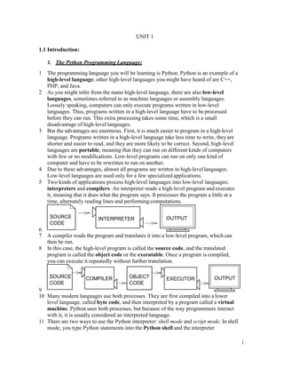
  • 1. 1 UNIT 1 1.1 Introduction: 1. The Python Programming Language: 1 The programming language you will be learning is Python. Python is an example of a high-level language; other high-level languages you might have heard of are C++, PHP, and Java. 2 As you might infer from the name high-level language, there are also low-level languages, sometimes referred to as machine languages or assembly languages. Loosely speaking, computers can only execute programs written in low-level languages. Thus, programs written in a high-level language have to be processed before they can run. This extra processing takes some time, which is a small disadvantage of high-level languages. 3 But the advantages are enormous. First, it is much easier to program in a high-level language. Programs written in a high-level language take less time to write, theyare shorter and easier to read, and they are more likely to be correct. Second, high-level languages are portable, meaning that they can run on different kinds of computers with few or no modifications. Low-level programs can run on only one kind of computer and have to be rewritten to run on another. 4 Due to these advantages, almost all programs are written in high-level languages. Low-level languages are used only for a few specialized applications. 5 Two kinds of applications process high-level languages into low-level languages: interpreters and compilers. An interpreter reads a high-level program and executes it, meaning that it does what the program says. It processes the program a little at a time, alternately reading lines and performing computations. 6 7 A compiler reads the program and translates it into a low-level program, which can then be run. 8 In this case, the high-level program is called the source code, and the translated program is called the object code or the executable. Once a program is compiled, you can execute it repeatedly without further translation. 9 10 Many modern languages use both processes. They are first compiled into a lower level language, called byte code, and then interpreted by a program called a virtual machine. Python uses both processes, but because of the way programmers interact with it, it is usually considered an interpreted language. 11 There are two ways to use the Python interpreter: shell mode and script mode. In shell mode, you type Python statements into the Python shell and the interpreter SOURCE CODE COMPILER EXECUTOR OUTPUTOBJECT CODE OUTPUTSOURCE CODE INTERPRETER
  • 2. 2 immediately prints the result. 12 In this course, we will be using an IDE (Integrated Development Environment)called IDLE. When you first start IDLE it will open an interpreter window.1 13 The first few lines identify the version of Python being used as well as a few other messages; you can safely ignore the lines about the firewall. Next there is a line identifying the version of IDLE. The last line starts with >>>, which is the Python prompt. The interpreter uses the prompt to indicate that it is ready for instructions. 14 If we type print 1 + 1 the interpreter will reply 2 and give us another prompt.2 15 >>> print 1 + 1 16 2 17 >>> 18 Alternatively, you can write a program in a file and use the interpreter to execute the contents of the file. Such a file is called a script. For example, we used the text editor in IDLE (but we could have used any text editor) to create a file named firstprogram.py with the following contents: 19 print 1 + 1 20 By convention, files that contain Python programs have names that end with .py. To execute the program we have to invoke the interpreter and tell it the name of the script: 21 $ python firstprogram.py 22 2 This example shows Python being run from a terminal (with $ representing the Unix prompt). In other development environments, the details of executing programs may differ. IDLE simplifies the whole process by presenting interpreter windows and a text editor within the same application. You can run a script in IDLE by either choosing Run → Run Module or pressing F5. Most programs are more interesting than this one. The examples in this book use both the Python interpreter and scripts. You will be able to tell which is intended since shell mode examples (i.e. entering lines directly into the interpreter) will always start with the Python prompt, >>>. Working in shell mode is convenient for testing short bits of code because you get immediate feedback. Think of it as scratch paper used to help you work out problems. Anything longer than a few lines should be put into a script so it can be saved for future use. 2. History of Python: Python was developed by Guido van Rossum in the late eighties and early nineties at the National Research Institute for Mathematics and Computer Science in the Netherlands. 1 You can also run the python interpreter by just entering the command python in a terminal. To exit from the interpreter type exit() and hit return, or press Ctrl-D on a new line. 2 The print statement is one of the changes between Python 2.x and Python 3.x. In Python 3.x, print is a function and not a
  • 3. 3 • Python is derived from many other languages, including ABC, Modula-3, C, C++, Algol-68, SmallTalk, and Unix shell and other scripting languages. • Python is copyrighted. Like Perl, Python source code is now available under the GNU General Public License (GPL). • Python is now maintained by a core development team at the institute, although Guido van Rossum still holds a vital role in directing its progress. • Python 1.0 was released in November 1994. In 2000, Python 2.0 was released. Python 2.7.11 is the latest edition of Python 2. • Meanwhile, Python 3.0 was released in 2008. Python 3 is not backward compatible with Python 2. The emphasis in Python 3 had been on the removal of duplicate programming constructs and modules so that "There should be one -- and preferably only one -- obvious way to do it." Python 3.5.1 is the latest version of Python 3. 3. Features of python: Python's features include- • Easy-to-learn: Python has few keywords, simple structure, and a clearly defined syntax. This allows a student to pick up the language quickly. • Easy-to-read: Python code is more clearly defined and visible to the eyes. • Easy-to-maintain: Python's source code is fairly easy-to-maintain. • A broad standard library: Python's bulk of the library is very portable and crossplatform compatible on UNIX, Windows, and Macintosh. • Interactive Mode: Python has support for an interactive mode, which allows interactive testing and debugging of snippets of code. • Portable: Python can run on a wide variety of hardware platforms and has the same interface on all platforms. • Extendable: You can add low-level modules to the Python interpreter. These modules enable programmers to add to or customize their tools to be more efficient. • Databases: Python provides interfaces to all major commercial databases. • GUI Programming: Python supports GUI applications that can be created and ported
  • 4. 4 to many system calls, libraries and windows systems, such as Windows MFC, Macintosh, and the X Window system of Unix. • Scalable: Python provides a better structure and support for large programs than shell scripting. Apart from the above-mentioned features, Python has a big list of good features. A few are listed below- • It supports functional and structured programming methods as well as OOP. • It can be used as a scripting language or can be compiled to byte-code for building large applications. • It provides very high-level dynamic data types and supports dynamic type checking. • It supports automatic garbage collection. • It can be easily integrated with C, C++, COM, ActiveX, CORBA, and Java. 4. Installing Python:
  • 5. 5 Windows platform Binaries of latest version of Python 3 (Python 3.5.1) are available on this download page The following different installation options are available. • Windows x86-64 embeddable zip file  Windows x86-64 executable installer  Windows x86-64 web-based installer • Windows x86 embeddable zip file Windows x86 executable installer • Windows x86 web-based installer Note:In order to install Python 3.5.1, minimum OS requirements are Windows 7 with SP1. For versions 3.0 to 3.4.x, Windows XP is acceptable. Linux platform Different flavors of Linux use different package managers for installation of new packages. On Ubuntu Linux, Python 3 is installed using the following command from the terminal. Installation from source Mac OS Download Mac OS installers from this URL:https://www.python.org/downloads/mac-osx/ • Mac OS X 64-bit/32-bit installer : python-3.5.1-macosx10.6.pkg • Mac OS X 32-bit i386/PPC installer : python-3.5.1-macosx10.5.pkg Double click this package file and follow the wizard instructions to install. The most up-to-date and current source code, binaries, documentation, news, etc., is available on the official website of Python: Download Gzipped source tarball from Python's download URL: https://www.python.org/ftp/python/3.5.1/Python- 3.5.1.tgz Extract the tarball tar xvfz Python-3.5.1.tgz Configure and Install: cd Python-3.5.1 ./configure --prefix=/opt/python3.5.1 make sudo make install $sudo apt-get install python3-minimal
  • 6. 6 Python Official Website : http://www.python.org/ You can download Python documentation from the following site. The documentation is available in HTML, PDF and PostScript formats. Python Documentation Website : www.python.org/doc/ Setting up PATH Programs and other executable files can be in many directories. Hence, the operating systems provide a search path that lists the directories that it searches for executables. The important features are- • The path is stored in an environment variable, which is a named string maintained by the operating system. This variable contains information available to the command shell and other programs. • The path variable is named as PATH in Unix or Path in Windows (Unix is casesensitive; Windows is not). • In Mac OS, the installer handles the path details. To invoke the Python interpreter from any particular directory, you must add the Python directory to your path. Setting Path at Unix/Linux To add the Python directory to the path for a particular session in Unix- • In the csh shell: type setenv PATH "$PATH:/usr/local/bin/python3" and pressEnter. • In the bash shell (Linux): type export PATH="$PATH:/usr/local/bin/python3" and press Enter. • In the sh or ksh shell: type PATH="$PATH:/usr/local/bin/python3" and pressEnter. Note: /usr/local/bin/python3 is the path of the Python directory. Setting Path at Windows To add the Python directory to the path for a particular session in Windows- At the command prompt : type path %path%;C:Python and press Enter.
  • 7. 7 Note: C:Python is the path of the Python directory. Python Environment Variables Here are important environment variables, which are recognized by Python- Variable Description PYTHONPATH It has a role similar to PATH. This variable tells the Python interpreter where to locate the module files imported into a program. It should include the Python source library directory and the directories containing Python source code. PYTHONPATH is sometimes, preset by the Python installer. PYTHONSTARTU P It contains the path of an initialization file containing Python source code. It is executed every time you start the interpreter. It is named as .pythonrc.py in Unix and it contains commands that load utilities or modify PYTHONPATH. PYTHONCASEOK It is used in Windows to instruct Python to find the first caseinsensitive match in an import statement. Set this variable to any value to activate it. PYTHONHOME It is an alternative module search path. It is usually embedded in the PYTHONSTARTUP or PYTHONPATH directories to make switching module libraries easy. 5. Running Python program: There are three different ways to start Python- (1) Interactive Interpreter You can start Python from Unix, DOS, or any other system that provides you a commandline interpreter or shell window. Enter python the command line.
  • 8. 8 Start coding right away in the interactive interpreter. Here is the list of all the available command line options- Option Description -d provide debug output -O generate optimized bytecode (resulting in .pyo files) -S do not run import site to look for Python paths on startup -v verbose output (detailed trace on import statements) -X disable class-based built-in exceptions (just use strings); obsolete starting with version 1.6 -c cmd run Python script sent in as cmd string file run Python script from given file (2) Script from the Command-line A Python script can be executed at the command line by invoking the interpreter on your application, as shown in the following example. Note: Be sure the file permission mode allows execution. (3) Integrated Development Environment $python python% C:>python # Unix/Linux or # Unix/Linux or # Windows/DOS $python script.py python% script.py C:>python script.py # Unix/Linux or # Unix/Linux or # Windows/DOS
  • 9. 9 You can run Python from a Graphical User Interface (GUI) environment as well, if you have a GUI application on your system that supports Python. • Unix: IDLE is the very first Unix IDE for Python. • Windows: PythonWin is the first Windows interface for Python and is an IDE with a GUI. • Macintosh: The Macintosh version of Python along with the IDLE IDE is available from the main website, downloadable as either MacBinary or BinHex'd files. If you are not able to set up the environment properly, then you can take the help of your system admin. Make sure the Python environment is properly set up and working perfectly fine. 6. Debugging: Programming is a complex process, and because it is done by human beings, programs often contain errors. For whimsical reasons, programming errors are called bugs and the process of tracking them down and correcting them is called debugging. Three kinds of errors can occur in a program: syntax errors, runtime errors, and semantic errors. It is useful to distinguish between them in order to track them down more quickly. Syntax errors Python can only execute a program if the program is syntactically correct; otherwise, the process fails and returns an error message. Syntax refers to the structure of a program and the rules about that structure. For example, in English, a sentence must begin with a capital letter and end with a period. this sentence contains a syntax error. So does this one For most readers, a few syntax errors are not a significant problem, which is why we can read the poetry of e. e. cummings without spewing error messages. Python is not so forgiving. If there is a single syntax error anywhere in your program, Python will print an error message and quit, and you will not be able to run your program. During the first few weeks of your programming career, you will probably spend a lot of time tracking down syntax errors. As you gain experience, though, you will make fewer syntax errors and find them faster. Runtime errors The second type of error is a runtime error, so called because the error does not appear until you run the program. These errors are also called exceptions because they usually indicate that something exceptional (and bad) has happened. Runtime errors are rare in the simple programs you will see in the first few chapters, so it might be a while before you encounter one.
  • 10. 10 Semantic errors The third type of error is the semantic error. If there is a semantic error in your program, it will run successfully, in the sense that the computer will not generate any error messages, but it will not do the right thing. It will do something else. Specifically, it will do what you told it to do. The problem is that the program you wrote is not the program you wanted to write. The meaning of the program (its semantics) is wrong. Identifying semantic errors can be tricky because it requires you to work backward by looking at the output of the program and trying to figure out what it is doing. One of the most important skills you will acquire is debugging. Although it can be frustrating, debugging is one of the most intellectually rich, challenging, and interesting parts of programming. In some ways, debugging is like detective work. You are confronted with clues, and you have to infer the processes and events that led to the results you see. Debugging is usually a trial and error process. Once you have an idea what is going wrong, you modify your program and try again. If your hypothesis was correct, then you can predict the result of the modification, and you take a step closer to a working program. If your hypothesis was wrong, you have to come up with a new one. As Sherlock Holmes pointed out, “When you have eliminated the impossible, whatever remains, however improbable, must be the truth.” (A. Conan Doyle, The Sign of Four ) For some people, programming and debugging are the same thing. That is, programming is the process of gradually debugging a program until it does what you want. The idea is that you should start with a program that does something and make small modifications, debugging them as you go, so that you always have a working program. For example, Linux is an operating system that contains thousands of lines of code, but it started out as a simple program Linus Torvalds used to explore the Intel 80386 chip. According to Larry Greenfield, one of Linus’s earlier projects was a program that would switch between printing AAAA and BBBB. This later evolved into Linux (The Linux Users’ Guide Beta Version 1). 7. Formal and Natural Languages: Natural languages are the languages that people speak, such as English, Spanish, and French. They were not designed by people (although people try to impose some order on them); they evolved naturally. Formal languages are languages that are designed by people for specific applications. For example, the notation that mathematicians use is a formal language that is particularly good at denoting relationships among numbers and symbols. Chemists use a formal
  • 11. 11 language to represent the chemical structure of molecules. And most importantly: Programming languages are formal languages that have been designed to express computations. Formal languages tend to have strict rules about syntax. For example, 3+3=6 is a syntactically correct mathematical statement, but 3=+6$ is not. H2O is a syntactically correct chemical name, but 2Zz is not. Syntax rules come in two flavors, pertaining to tokens and structure. Tokens are the basic elements of the language, such as words, numbers, and chemical elements. One of the problems with 3=+6$ is that $ is not a legal token in mathematics (at least as far as we know). Similarly, 2Zz is not legal because there is no element with the abbreviation Zz. The second type of syntax rule pertains to the structure of a statement— that is, the way the tokens are arranged. The statement 3=+6$ is structurally illegal because you can’t place a plus sign immediately after an equal sign. Similarly, molecular formulas have to have subscripts after the element name, not before. When you read a sentence in English or a statement in a formal language, you have to figure out what the structure of the sentence is (although in a natural language you do this subconsciously). This process is called parsing. For example, when you hear the sentence, “The brown dog barked”, you understand that the brown dog is the subject and barked is the verb. Once you have parsed a sentence, you can figure out what it means, or the semantics of the sentence. Assuming that you know what a dog is and what it means to bark, you will understand the general implication of this sentence. Although formal and natural languages have many features in common—tokens, structure, syntax, and semantics—there are many differences: ambiguity: Natural languages are full of ambiguity, which people deal with by using contextual clues and other information. Formal languages are designed to be nearly or completely unambiguous, which means that any statement has exactly one meaning, regardless of context. redundancy: In order to make up for ambiguity and reduce misunderstandings, natural languages employ lots of redundancy. As a result, they are often verbose. Formal languages are less redundant and more concise. literalness: Natural languages are full of idiom and metaphor. If someone says, “The penny dropped”, there is probably no penny and nothing dropped. Formal languages mean exactly what they say. People who grow up speaking a natural language—everyone—often have a hard time adjusting to formal languages. In some ways, the difference between formal and natural language is like the difference between poetry and prose, but more so: Poetry: Words are used for their sounds as well as for their meaning, and the whole poem together creates an effect or emotional response. Ambiguity is not only common but often deliberate. Prose: The literal meaning of words is more important, and the structure contributes
  • 12. 12 more meaning. Prose is more amenable to analysis than poetry but still often ambiguous. Programs: The meaning of a computer program is unambiguous and literal, and can be understood entirely by analysis of the tokens and structure. Here are some suggestions for reading programs (and other formal languages). First, remember that formal languages are much more dense than natural languages, so it takes longer to read them. Also, the structure is very important, so it is usually not a good idea to read from top to bottom, left to right. Instead, learn to parse the program in your head, identifying the tokens and interpreting the structure. Finally, the details matter. Little things like spelling errors and bad punctuation, which you can get away with in natural languages, can make a big difference in a formal language. 8. The Difference Between Brackets, Braces, and Parentheses: Braces are used for different purposes. If you just want a list to contain some elements and organize them by index numbers (starting from 0), just use the [] and add elements as necessary. {} are special in that you can give custom id's to values like a = {"John": 14}. Now, instead of making a list with ages and remembering whose age is where, you can just access John's age by a["John"]. The [] is called a list and {} is called a dictionary (in Python). Dictionaries are basically a convenient form of list which allow you to access data in a much easier way. However, there is a catch to dictionaries. Many times, the data that you put in the dictionary doesn't stay in the same order as before. Hence, when you go through each value one by one, it won't be in the order you expect. There is a special dictionary to get around this, but you have to add this line from collections import OrderedDict and replace {} with OrderedDict(). But, I don't think you will need to worry about that for now. 1.2 Variables and Expressions: 1. Values and Types: A value is one of the fundamental things—like a letter or a number—that a program manipulates. The values we have seen so far are 2 (the result when we added 1 + 1), and “Hello, World!”. These values belong to different types: 2 is an integer, and “Hello, World!” is a string. You (and the interpreter) can identify strings because they are enclosed in quotation marks. The print statement also works for integers. >>> print(4) 4 If you are not sure what type a value has, the interpreter can tell you. >>> type("Hello, World!")
  • 13. 13 Strings belong to the type str and integers belong to the type int. Less obviously, numbers with a decimal point belong to a type called float, because these numbers are represented in a format called floating-point. What about values like “17” and “3.2”? They look like numbers, but they are in quotation marks like strings. <class ’str’> They’re strings. Strings in Python can be enclosed in either single quotes (’) or double quotes (”): Double quoted strings can contain single quotes inside them, as in "What’s your name?", and single quoted strings can have double quotes inside them, as in ’The cat said "Meow!"’. When you type a large integer, you might be tempted to use commas between groups of three digits, as in 1,000,000. 2. Variables: One of the most powerful features of a programming language is the ability to manipulate variables. A variable is a name that refers to a value. The assignment statement creates new variables and assigns them values: <class ’str’> >>> type(17) < class ’int’> >>> type(3.2) <class ’float’> >>> type("17") <class ’str’> >>> type("3.2") >>> type(’This is a string.’) <class ’str’> >>> type("And so is this.") <class ’str’> >>> message = "What’s your name?" >>> n = 17 >>> pi = 3.14159
  • 14. 14 This example makes three assignments. The first assigns the string "What’s your name?" to a new variable named message. The second assigns the integer 17 to n, and the third assigns the floating-point number 3.14159 to pi. The assignment operator, =, should not be confused with an equals sign (even though it uses the same character). Assignment operators link a name, on the left hand side of the operator, with a value, on the right hand side. This is why you will get an error if you enter: A common way to represent variables on paper is to write the name with an arrow pointing to the variable’s value. This kind of figure is called a state diagram because it shows what state each of the variables is in (think of it as the variable’s state of mind). This diagram shows the result of the assignment statements: messag e n pi "What’s your name?" 17 3.14159 The print statement also works with variables. In each case the result is the value of the variable. Variables also have types; again, we can ask the interpreter what they are. The type of a variable is the type (or kind) of value it refers to. >>> 17 = n >>>print (message) What’s your name? >>> print (n) 17 >>> print (pi) 3.14159 >>> type(message) <class ’str’> >>> type(n) < class ’int’> >>> type(pi) < class ’float’>
  • 15. 15 3. Variable names and keywords: Programmers generally choose names for their variables that are meaningful—they document what the variable is used for. Variable names can be arbitrarily long. They can contain both letters and numbers, but they have to begin with a letter. Although it is legal to use uppercase letters, by convention we don’t. If you do, remember that case matters. Bruce and bruce are different variables. The underscore character ( ) can appear in a name. It is often used in names with multiple words, such as myname or priceofteainchina. If you give a variable an illegal name, you get a syntax error: 76trombones is illegal because it does not begin with a letter. more$ is illegal because it contains an illegal character, the dollar sign. But what’s wrong with class? It turns out that class is one of the Python keywords. Keywords define the language’s rules and structure, and they cannot be used as variable names. Python has thirty-one keywords: and del from not while as elif global or with assert else if pass yield break except import print class exec in raise continue finally is return def for lambda try 4. Type conversion: Sometimes, you may need to perform conversions between the built-in types. To convert between types, you simply use the type-name as a function. There are several built-in functions to perform conversion from one data type to another. >>> 76trombones = "big parade" SyntaxError: invalid syntax >>> more$ = 1000000 SyntaxError: invalid syntax >>> class = "COMP150" SyntaxError: invalid syntax
  • 16. 16 These functions return a new object representing the converted value. Function Description int(x [,base]) Converts x to an integer. The base specifies the base if x is a string. float(x) Converts x to a floating-point number. complex(real [,imag]) Creates a complex number. str(x) Converts object x to a string representation. repr(x) Converts object x to an expression string. eval(str) Evaluates a string and returns an object. tuple(s) Converts s to a tuple. list(s) Converts s to a list. set(s) Converts s to a set. dict(d) Creates a dictionary. d must be a sequence of (key,value) tuples. frozenset(s) Converts s to a frozen set. chr(x) Converts an integer to a character. unichr(x) Converts an integer to a Unicode character.
  • 17. 17 ord(x) Converts a single character to its integer value. hex(x) Converts an integer to a hexadecimal string. oct(x) Converts an integer to an octal string. 5. Operators and Operands: Operators are special symbols that represent computations like addition and multiplication. The values the operator uses are called operands. The following are all legal Python expressions whose meaning is more or less clear: The symbols +, -, *, /, have the usual mathematical meanings. The symbol, **, is the exponentiation operator. The statement, 5 ** 2, means 5 to the power of 2, or 5 squared in this case. Python also uses parentheses for grouping, so we can force operations to be done in a certain order just like we can in mathematics. When a variable name appears in the place of an operand, it is replaced with its value before the operation is performed. Addition, subtraction, multiplication, and exponentiation all do what you expect, but you might be surprised by division. The following operation has an unexpected result: The value of minute is 59, and 59 divided by 60 is 0.98333, not 0. The reason for the discrepancy is that Python is performing integer division3 . When both of the operands are integers, the result must also be an integer, and by convention, integer division always rounds down, even in cases like this where the next integer is very close. A possible solution to this problem is to calculate a percentage rather than a fraction: 20 + 32 hour - 1 hour * 60 + minute minute / 60 5 ** 2 (5 + 9) * (15 - 7) >>> minute = 59 >>> minute / 60 0 .9833333333333333 >>> minute * 100 / 60
  • 18. 18 Operators are special symbols that represent computations like addition and multiplication. The values the operator uses are called operands. The following are all legal Python expressions whose meaning is more or less clear: The symbols +, -, *, /, have the usual mathematical meanings. The symbol, **, is the exponentiation operator. The statement, 5 ** 2, means 5 to the power of 2, or 5 squared in this case. Python also uses parentheses for grouping, so we can force operations to be done in a certain order just like we can in mathematics. When a variable name appears in the place of an operand, it is replaced with its value before the operation is performed. Addition, subtraction, multiplication, and exponentiation all do what you expect, but you might be surprised by division. The following operation has an unexpected result: The value of minute is 59, and 59 divided by 60 is 0.98333, not 0. The reason for the discrepancy is that Python is performing integer division4 . When both of the operands are integers, the result must also be an integer, and by convention, integer division always rounds down, even in cases like this where the next integer is very close. A possible solution to this problem is to calculate a percentage rather than a fraction: Again the result is rounded down, but at least now the answer is approximately correct. Another alternative is to use floating-point division. 6. Expressions: An expression is a combination of values, variables, and operators. If you type an expression on the command line, the interpreter evaluates it and displays the result: 20 + 32 hour - 1 hour * 60 + minute minute / 60 5 ** 2 (5 + 9) * (15 - 7) >>> minute = 59 >>> minute / 60 0 .9833333333333333 >>> minute * 100 / 60 98.33333333333333 >>> 1 + 1 2
  • 19. 19 The evaluation of an expression produces a value, which is why expressions can appear on the right hand side of assignment statements. A value all by itself is a simple expression, and so is a variable. Confusingly, evaluating an expression is not quite the same thing as printing a value. >>> message = "What’s your name?" >>> message "What’s your name?" >>> print(message) What’s your name? When the Python shell displays the value of an expression, it uses the same format you would use to enter a value. In the case of strings, that means that it includes the quotation marks. But the print statement prints the value of the expression, which in this case is the contents of the string. In a script, an expression all by itself is a legal statement, but it doesn’t do anything. The script 17 3.2 "Hello, World!" 1 + 1 produces no output at all. How would you change the script to display the values of these four expressions? 7. Interactive Mode and Script Mode: Interactive Mode Programming Invoking the interpreter without passing a script file as a parameter brings up the following prompt- >>> 17 17 >>> x 2
  • 20. 20 $ python Python 3.3.2 (default, Dec 10 2013, 11:35:01) [GCC 4.6.3] on Linux Type "help", "copyright", "credits", or "license" for more information. >>> On Windows: Python 3.4.3 (v3.4.3:9b73f1c3e601, Feb 24 2015, 22:43:06) [MSC v.1600 32 bit (Intel)] on win32 Type "copyright", "credits" or "license()" for more information. >>> Type the following text at the Python prompt and press Enter- If you are running the older version of Python (Python 2.x), use of parenthesis as inprint function is optional. This produces the following result- Script Mode Programming Invoking the interpreter with a script parameter begins execution of the script and continues until the script is finished. When the script is finished, the interpreter is no longer active. Let us write a simple Python program in a script. Python files have the extension.py. Type the following source code in a test.py file- We assume that you have the Python interpreter set in PATH variable. Now, try to run this program as follows- On Linux This produces the following result- On Windows This produces the following result- >>> print ("Hello, Python!") Hello, Python! print ("Hello, Python!") $ python test.py Hello, Python! C:Python34>Python test.py
  • 21. 21 Let us try another way to execute a Python script in Linux. Here is the modified test.py file- We assume that you have Python interpreter available in the /usr/bin directory. Now, try to run this program as follows- This produces the following result- Order of Operations: When more than one operator appears in an expression, the order of evaluation depends on the rules of precedence. Python follows the same precedence rules for its mathematical operators that mathematics does. The acronym PEMDAS is a useful way to remember the order of operations: 1. Parentheses have the highest precedence and can be used to force an expression to evaluate in the order you want. Since expressions in parentheses are evaluated first, 2*(3-1) is 4, and (1+1)**(5-2) is 8. You can also use parentheses to make an expression easier to read, as in (minute*100)/60, even though it doesn’t change the result. 2. Exponentiation has the next highest precedence, so 2**1+1 is 3 and not 4, and 3*1**3 is 3 and not 27. 3. Multiplication and Division have the same precedence, which is higher than Addition and Subtraction, which also have the same precedence. So 2*3-1 yields 5 rather than 4, and 2/3-1 is -1, not 1 (remember that in integer division, 2/3=0). Operators with the same precedence are evaluated from left to right. So in the expression minute*100/60, the multiplication happens first, yielding 5900/60, which in turn yields 98. If the operations had been evaluated from right to left, the result would have been 59*1, which is 59, which is wrong. Similarly, in evaluating 17-4-3, Hello, Python! #!/usr/bin/python3 print ("Hello, Python!") $ chmod +x test.py # This is to make file executable $./test.py Hello, Python!
  • 22. 22 17-4 is evaluated first. If in doubt, use parentheses. 1.3 Conditional Statements: 1. IF statement: The IF statement is similar to that of other languages. The if statement contains a logical expression using which the data is compared and a decision is made based on the result of the comparison. Syntax If the boolean expression evaluates to TRUE, then the block of statement(s) inside the if statement is executed. In Python, statements in a block are uniformly indented after the : symbol. If boolean expression evaluates to FALSE, then the first set of code after the end of block is executed. if expression: statement(s)
  • 23. 23 Flow Diagram nested if statements You can use one if or else if statement inside another if or else if statement(s). Example When the above code is executed, it produces the following result − num = 3 if num > 0: print(num, "is a positive number.") print("This is always printed.") num = -1 if num > 0: print(num, "is a positive number.") print("This is also always printed.")
  • 24. 24 3 is a positive number. This is always printed. In the above example, num > 0 is the test expression. The body of if is executed only if this evaluates to True. When variable num is equal to 3, test expression is true and body inside body of if is executed. If variable num is equal to -1, test expression is false and body inside body of if is skipped. The print() statement falls outside of the if block (unindented). Hence, it is executed regardless of the test expression. 2. IF ELSE Statements An else statement can be combined with an if statement. An else statement contains a block of code that executes if the conditional expression in the if statement resolves to 0 or a FALSE value. The else statement is an optional statement and there could be at the most only one else statement following if. Syntax The syntax of the if...else statement is- if expression: statement(s) else: statement(s) Flow Diagram
  • 25. 25 Positive or Zero Example # Program checks if the number is positive or negative # And displays an appropriate message num = 3 # Try these two variations as well. # num = -5 # num = 0 if num >= 0: print("Positive or Zero") else: print("Negative number") In the above example, when num is equal to 3, the test expression is true and body of if is executed and body of else is skipped. If num is equal to -5, the test expression is false and body of else is executed and body
  • 26. 26 of if is skipped. 3. Nested IF -ELSE Statements There may be a situation when you want to check for another condition after a condition resolves to true. In such a situation, you can use the nested if construct. In a nested if construct, you can have an if...elif...else construct inside another if...elif...else construct. Syntax The syntax of the nested if...elif...else construct may be- if expression1: statement(s) if expression2: statement(s) elif expression3: statement(s) else statement(s) elif expression4: statement(s) else: statement(s)
  • 27. 27 Example When the above code is executed, it produces the following result- # !/usr/bin/python3 # In this program, we input a number # check if the number is positive or # negative or zero and display # an appropriate message # This time we use nested if num = float(input("Enter a number: ")) if num >= 0: if num == 0: print("Zero") else: print("Positive number") else: print("Negative number") num=int(input("enter number")) Output 1 Enter a number: 5 Positive number Output 2 Enter a number: -1 Negative number Output 3 Enter a number: 0 Zero Divisible by 3 and 2 enter number5
  • 28. 28 not Divisible by 2 not divisible by 3 1.4 Looping: 1. For: The for loop in Python is used to iterate over a sequence (list, tuple, string) or other iterable objects. Iterating over a sequence is called traversal. Syntax of for Loop for val in sequence: Body of for Here, val is the variable that takes the value of the item inside the sequence on each iteration. Loop continues until we reach the last item in the sequence. The body of for loop is separated from the rest of the code using indentation. Flowchart of for Loop
  • 29. 29 Example: Python for Loop # Program to find the sum of all numbers stored in a list # List of numbers numbers = [6, 5, 3, 8, 4, 2, 5, 4, 11] # variable to store the sum sum = 0 # iterate over the list for val in numbers:
  • 30. 30 sum = sum+val # Output: The sum is 48 print("The sum is", sum) when you run the program, the output will be: The sum is 48 2. While Loop The while loop in Python is used to iterate over a block of code as long as the test expression (condition) is true. We generally use this loop when we don't know beforehand, the number of times to iterate. Syntax of while Loop in Python while test_expression: Body of while In while loop, test expression is checked first. The body of the loop is entered only if the test_expression evaluates to True. After one iteration, the test expression is checked again. This process continues until the test_expression evaluates to False. In Python, the body of the while loop is determined through indentation. Body starts with indentation and the first unindented line marks the end. Python interprets any non-zero value as True. None and 0 are interpreted as False. Flowchart of while Loop
  • 31. 31 Example: Python while Loop # Program to add natural # numbers upto # sum = 1+2+3+...+n # To take input from the user, # n = int(input("Enter n: ")) n = 10 # initialize sum and counter
  • 32. 32 When you run the program, the output will be: In the above program, the test expression will be True as long as our counter variable i is less than or equal to n (10 in our program). We need to increase the value of counter variable in the body of the loop. This is very important (and mostly forgotten). Failing to do so will result in an infinite loop (never ending loop). Finally the result is displayed. 3. Nested loops: Python programming language allows to use one loop inside another loop. Following section shows few examples to illustrate the concept. sum = 0 i = 1 while i <= n: sum = sum + i i = i+1 # update counter # print the sum print("The sum is", sum) Enter n: 10 The sum is 55
  • 33. 33 Python Nested if Example # In this program, we input a number # check if the number is positive or # negative or zero and display # an appropriate message # This time we use nested if num = float(input("Enter a number: ")) if num >= 0: if num == 0: print("Zero") else: print("Positive number") else: print("Negative number") Output 1 Enter a number: 5 Positive number Output 2 Enter a number: -1 Negative number Output 3 Enter a number: 0 Zero 1.5 Control statements: 1. Terminating loops: The break statement terminates the loop containing it. Control of the program flows to the statement immediately after the body of the loop.
  • 34. 34 If break statement is inside a nested loop (loop inside another loop), break will terminate the innermost loop. Syntax of break Flowchart of break break
  • 35. 35 Example: Python break Output In this program, we iterate through the "string" sequence. We check if the letter is "i", upon # Use of break statement inside loop for val in "string": if val == "i": break print(val) print("The end") s t r The end
  • 36. 36 which we break from the loop. Hence, we see in our output that all the letters up till "i" gets printed. After that, the loop terminates. 2. Skipping specific conditions: The continue statement is used to skip the rest of the code inside a loop for the current iteration only. Loop does not terminate but continues on with the next iteration. Syntax of Continue continue Flowchart of continue The working of continue statement in for and while loop is shown below.
  • 37. 37 Example: Python continue Output # Program to show the use of continue statement inside loops for val in "string": if val == "i": continue print(val) print("The end") s t
  • 38. 38 This program is same as the above example except the break statement has been replaced with continue. We continue with the loop, if the string is "i", not executing the rest of the block. Hence, we see in our output that all the letters except "i" gets printed. r n g The end
  • 39. 39
  • 40. 40 UNIT 2 FUNCTIONS : 2.1 Composing Expressions So far, we have looked at the elements of a program—variables, expressions, and statements —in isolation, without talking about how to combine them. One of the most useful features of programming languages is their ability to take small building blocks and compose them. For example, we know how to add numbers and we know how to print; it turns out we can do both at the same time: In reality, the addition has to happen before the printing, so the actions aren’t actually happening at the same time. The point is that any expression involving numbers, strings, and variables can follow print: You can also put arbitrary expressions on the right-hand side of an assignment statement: This ability may not seem impressive now, but you will see other examples where the composition makes it possible to express complex computations neatly and concisely. Warning: There are limits on where you can use certain expressions. For example, left-hand side of an assignment statement has to be a variable name, not an expression. So, the following is illegal: 3.2 Function calls Many common tasks come up time and time again when programming. Instead of requiring you to constantly reinvent the wheel, Python has a number of built-in features which you can use. Including so much ready to use code is sometimes >>> print(17 + 3) 20 >>> hour = 21 >>> minute = 1 >>> print("Number of minutes since midnight: ",hour * 60 + minute) Number of minutes since midnight: 1261 >>> percentage = (minute * 100) / 60 >>> percentage 1.6666666666666667 >>> print(percentage) 1.6666666666666667 >>> minute+1 = hour File "<stdin>", line 1 SyntaxError: can't assign to operator
  • 41. 41 referred to as a ’batteries included’ philosophy. Python comes with just under fifty (of which we’ll be only using about a dozen) and the simplest way to use this prewritten code is via function calls. The syntax of a function call is simply FUNCTION NAME(ARGUMENTS) Not all functions take an argument, and some take more than one (in which case the arguments are separated by commas). You have already seen an example of a function call: >>> type("Hello,World") <class 'str'> >>> type(17) <class 'int'> The name of the function is type, and it displays the type of a value or variable. The value or variable, which is called the argument of the function, has to be enclosed in parentheses. It is common to say that a function “takes” an argument and “returns” a result. The result is called the return value. We can assign the return value to a variable: Another useful function is len. It takes a Python sequence as an argument. The only Python sequence we have met so far is a string. A string is a sequence of characters. For a string argument, len returns the number of characters the string contains. The len function can only be used on sequences. Trying to use it on a number, for example, results in an error. 2.3 Type Conversion Functions : Each Python type comes with a built-in function that attempts to convert values of another type into that type. The int(ARGUMENT) function, for example, takes any value and converts it to an integer, if possible, or complains otherwise: >>> result = type(17) >>> print(result) <class 'int'> >>> my_str = "Hello world" >>> len(my_str) 11 >>> len(3) Traceback (most recent call last): File "<stdin>", line 1, in <module> TypeError: object of type 'int' has no len() >>> int("32")
  • 42. 42 The int function can also convert floating-point values to integers, but note that it truncates the fractional part: The float(ARGUMENT) function converts integers and strings to floating-point numbers: >>> float(32) 32.0 >>> float("3.14159") 3.14159 >>> float(1) 1.0 It may seem odd that Python distinguishes the integer value 1 from the floating-point value 1.0. They may represent the same number, but they belong to different types as they are represented differently inside the computer. The str(ARGUMENT) function converts any argument to type string: The str(ARGUMENT) function will work with any value and convert it into a string. Note: True is a predefined value in Python; true is not. 2.4 Math Functions : Python includes following functions that perform mathematical calculations. 32 >>> int("Hello") Traceback (most recent call last): File "<stdin>", line 1, in <module> ValueError: invalid literal for int() with base 10: 'Hello' >>> int(-2.3) -2 >>> int(3.99999) 3 >>> int("42") 42 >>> int(1.0) 1 >>> str(32) '32' >>> str(3.14149) '3.14149' >>> str(True) 'True' >>> str(true) Traceback (most recent call last): File "<stdin>", line 1, in <module> NameError: name 'true' is not defined
  • 43. 43 Function Returns ( description ) abs(x) The absolute value of x: the (positive) distance between x and zero. ceil(x) The ceiling of x: the smallest integer not less than x cmp(x, y) -1 if x < y, 0 if x == y, or 1 if x > y exp(x) The exponential of x: ex fabs(x) The absolute value of x. floor(x) The floor of x: the largest integer not greater than x log(x) The natural logarithm of x, for x> 0 log10(x) The base-10 logarithm of x for x> 0. max(x1, x2,...) The largest of its arguments: the value closest to positive infinity min(x1, x2,...) The smallest of its arguments: the value closest to negative infinity modf(x) The fractional and integer parts of x in a two-item tuple. Both parts have the same sign as x. The integer part is returned as a float. pow(x, y) The value of x**y. round(x [,n]) x rounded to n digits from the decimal point. Python rounds away from zero as a tie-breaker: round(0.5) is 1.0 and round(-0.5) is -1.0. Number abs() Method : Description: The abs() method returns the absolute value of x i.e. the positive distance between x and zero. Syntax : Following is the syntax for abs() method- abs(x) Parameters : x - This is a numeric expression. Return : This method returns the absolute value of x. The following example shows the usage of the abs() method. print ("abs(-45) : ", abs(-45)) print ("abs(100.12) : ", abs(100.12))
  • 44. 44 When we run the above program, it produces the following result- Number ceil() Method : Description: The ceil() method returns the ceiling value of x i.e. the smallest integer not less than x. Syntax: Following is the syntax for the ceil() method import math math.ceil( x ) Note: This function is not accessible directly, so we need to import math module and then we need to call this function using the math static object. Parameters x - This is a numeric expression. Return Value This method returns the smallest integer not less than x. Example The following example shows the usage of the ceil() method. When we run the above program, it produces the following result Number exp() Method Description The exp() method returns exponential of x: ex. Syntax Following is the syntax for the exp() method Note: This function is not accessible directly. Therefore, we need to import the math module and then we need to call this function using the math static object. Parameters X - This is a numeric expression. Return Value This method returns exponential of x: ex. abs(-45): 45 abs(100.12) : 100.12 import math # This will import math module print ("math.ceil(-45.17) : ", math.ceil(-45.17)) print ("math.ceil(100.12) : ", math.ceil(100.12)) print ("math.ceil(100.72) : ", math.ceil(100.72)) print ("math.ceil(math.pi) : ", math.ceil(math.pi)) math.ceil(-45.17) : -45 math.ceil(100.12) : 101 math.ceil(100.72) : 101 math.ceil(math.pi) : 4 import math math.exp( x )
  • 45. 45 Example The following example shows the usage of exp() method. When we run the above program, it produces the following result Number fabs() Method Description The fabs() method returns the absolute value of x. Although similar to the abs() function, there are differences between the two functions. They are- • abs() is a built in function whereas fabs() is defined in math module. • fabs() function works only on float and integer whereas abs() works with complex number also. Syntax Following is the syntax for the fabs() method Note: This function is not accessible directly, so we need to import the math module and then we need to call this function using the math static object. Parameters x - This is a numeric value. Return Value This method returns the absolute value of x. Example The following example shows the usage of the fabs() method. When we run the above program, it produces following result import math # This will import math module print ("math.exp(-45.17) : ", math.exp(-45.17)) print ("math.exp(100.12) : ", math.exp(100.12)) print ("math.exp(100.72) : ", math.exp(100.72)) print ("math.exp(math.pi) : ", math.exp(math.pi)) math.exp(-45.17) : 2.4150062132629406e-20 math.exp(100.12) : 3.0308436140742566e+43 math.exp(100.72) : 5.522557130248187e+43 math.exp(math.pi) : 23.140692632779267 import math math.fabs( x ) import math # This will import math module print ("math.fabs(-45.17) : ", math.fabs(-45.17)) print ("math.fabs(100.12) : ", math.fabs(100.12)) print ("math.fabs(100.72) : ", math.fabs(100.72)) print ("math.fabs(math.pi) : ", math.fabs(math.pi)) math.fabs(-45.17) : 45.17
  • 46. 46 Number floor() Method Description The floor() method returns the floor of x i.e. the largest integer not greater than x. Syntax Following is the syntax for the floor() method Note: This function is not accessible directly, so we need to import the math module and then we need to call this function using the math static object. Parameters x - This is a numeric expression. Return Value This method returns the largest integer not greater than x. The following example shows the usage of the floor() method. When we run the above program, it produces the following result Number log() Method Description The log() method returns the natural logarithm of x, for x > 0. Syntax Following is the syntax for the log() method Note: This function is not accessible directly, so we need to import the math module and then we need to call this function using the math static object. Parameters math.fabs(100.12) : 100.12 math.fabs(100.72) : 100.72 math.fabs(math.pi) : 3.141592653589793 import math math.floor( x ) import math # This will import math module print ("math.floor(-45.17) : ", math.floor(-45.17)) print ("math.floor(100.12) : ", math.floor(100.12)) print ("math.floor(100.72) : ", math.floor(100.72)) print ("math.floor(math.pi) : ", math.floor(math.pi)) math.floor(-45.17) : -46 math.floor(100.12) : 100 math.floor(100.72) : 100 math.floor(math.pi) : 3 import math math.log( x )
  • 47. 47 x - This is a numeric expression. Return Value This method returns natural logarithm of x, for x > 0. Example The following example shows the usage of the log() method. When we run the above program, it produces the following result Number log10() Method Description The log10() method returns base-10 logarithm of x for x > 0. Syntax Following is the syntax for log10() method Note: This function is not accessible directly, so we need to import the math module and then we need to call this function using the math static object. Parameters x - This is a numeric expression. Return Value This method returns the base-10 logarithm of x for x > 0. Example The following example shows the usage of the log10() method. import math # This will import math module print ("math.log10(100.12) : ", math.log10(100.12)) print ("math.log10(100.72) : ", math.log10(100.72)) print ("math.log10(119) : ", math.log10(119)) print ("math.log10(math.pi) : ", math.log10(math.pi)) When we run the above program, it produces the following result Number max() Method Description import math # This will import math module print ("math.log(100.12) : ", math.log(100.12)) print ("math.log(100.72) : ", math.log(100.72)) print ("math.log(math.pi) : ", math.log(math.pi)) math.log(100.12) : 4.6063694665635735 math.log(100.72) : 4.612344389736092 math.log(math.pi) : 1.1447298858494002 import math math.log10( x ) math.log10(100.12) : 2.0005208409361854 math.log10(100.72) : 2.003115717099806 math.log10(119) : 2.0755469613925306 math.log10(math.pi) : 0.49714987269413385
  • 48. 48 The max() method returns the largest of its arguments i.e. the value closest to positive infinity. Syntax Following is the syntax for max() method Parameters • x - This is a numeric expression. • y - This is also a numeric expression. • z - This is also a numeric expression. Return Value This method returns the largest of its arguments. Example The following example shows the usage of the max() method. When we run the above program, it produces the following result Number min() Method Description The method min() returns the smallest of its arguments i.e. the value closest to negative infinity. Syntax Following is the syntax for the min() method Parameters • x - This is a numeric expression. • y - This is also a numeric expression. • z - This is also a numeric expression. Return Value This method returns the smallest of its arguments. Example The following example shows the usage of the min() method. max(x, y, z, .... ) print ("max(80, 100, 1000) : ", max(80, 100, 1000)) print ("max(-20, 100, 400) : ", max(-20, 100, 400)) print ("max(-80, -20, -10) : ", max(-80, -20, -10)) print ("max(0, 100, -400) : ", max(0, 100, -400)) max( 80, 100, 1000) : 1000 max(-20, 100, 400) : 400 max(-80, -20, -10) : -10 max(0, 100, -400) : 100 min(x, y, z, .... ) print ("min(80, 100, 1000) : ", min(80, 100, 1000))
  • 49. 49 When we run the above program, it produces the following result Number modf() Method Description The modf() method returns the fractional and integer parts of x in a two-item tuple. Both parts have the same sign as x. The integer part is returned as a float. Syntax Following is the syntax for the modf() method Note: This function is not accessible directly, so we need to import the math module and then we need to call this function using the math static object. Parameters x - This is a numeric expression. Return Value This method returns the fractional and integer parts of x in a two-item tuple. Both the parts have the same sign as x. The integer part is returned as a float. Example The following example shows the usage of the modf() method. When we run the above program, it produces the following result Number pow() Method Return Value This method returns the value of xy. Example The following example shows the usage of the pow() method. print ("min(-20, 100, 400) : ", min(-20, 100, 400)) print ("min(-80, -20, -10) : ", min(-80, -20, -10)) print ("min(0, 100, -400) : ", min(0, 100, -400)) min(80, 100, 1000) : 80 min(-20, 100, 400) : -20 min(-80, -20, -10) : -80 min(0, 100, -400) : -400 import math math.modf( x ) import math # This will import math module print ("math.modf(100.12) : ", math.modf(100.12)) print ("math.modf(100.72) : ", math.modf(100.72)) print ("math.modf(119) : ", math.modf(119)) print ("math.modf(math.pi) : ", math.modf(math.pi)) math.modf(100.12) : (0.12000000000000455, 100.0) math.modf(100.72) : (0.7199999999999989, 100.0) math.modf(119) : (0.0, 119.0) math.modf(math.pi) : (0.14159265358979312, 3.0)
  • 50. 50 When we run the above program, it produces the following result Number round() Method Description round() is a built-in function in Python. It returns x rounded to n digits from the decimal point. Syntax Following is the syntax for the round() method Parameters • x - This is a numeric expression. • n - Represents number of digits from decimal point up to which x is to be rounded. Default is 0. Return Value This method returns x rounded to n digits from the decimal point. Example The following example shows the usage of round() method When we run the above program, it produces the following result Number sqrt() Method Description import math # This will import math module print ("math.pow(100, 2) : ", math.pow(100, 2)) print ("math.pow(100, -2) : ", math.pow(100, -2)) print ("math.pow(2, 4) : ", math.pow(2, 4)) print ("math.pow(3, 0) : ", math.pow(3, 0)) math. pow(100, 2) : 10000.0 math.pow(100, -2) : 0.0001 math.pow(2, 4) : 16.0 math.pow(3, 0) : 1.0 round(x [, n] ) print ("round(70.23456) : ", round(70.23456)) print ("round(56.659,1) : ", round(56.659,1)) print ("round(80.264, 2) : ", round(80.264, 2)) print ("round(100.000056, 3) : ", round(100.000056, 3)) print ("round(-100.000056, 3) : ", round(-100.000056, 3)) round(70.23456) : 70 round(56.659,1) : 56.7 round(80.264, 2) : 80.26 round(100.000056, 3) : 100.0 round(-100.000056, 3) : -100.0
  • 51. 51 The sqrt() method returns the square root of x for x > 0. Syntax Following is the syntax for sqrt() method Note: This function is not accessible directly, so we need to import the math module and then we need to call this function using the math static object. Parameters x - This is a numeric expression. Return Value This method returns square root of x for x > 0. Example The following example shows the usage of sqrt() method. When we run the above program, it produces the following result 2.5 Function Composition : Just as with mathematical functions, Python functions can be composed, meaning that you use the result of one function as the input to another. In the first example, abs(-7) evaluates to 7, which then becomes the argument to print twice. In the second example we have two levels of composition, since abs(- 11) is first evaluated to 11 before max(3, 1, 11, 7) is evaluated to 11 and (11) print_twice then displays the result. We can also use a variable as an argument: import math math.sqrt( x ) import math # This will import math module print ("math.sqrt(100) : ", math.sqrt(100)) print ("math.sqrt(7) : ", math.sqrt(7)) print ("math.sqrt(math.pi) : ", math.sqrt(math.pi)) math.sqrt(100) : 10.0 math.sqrt(7) : 2.6457513110645907 math.sqrt(math.pi) : 1.7724538509055159 >>> def print_twice(some_variable_name): ... print(some_variable_name, some_variable_name) ... >>> print_twice(abs(-7)) 7 7 >>> print_twice(max(3,1,abs(-11),7)) 11 11
  • 52. 52 Notice something very important here. The name of the variable we pass as an argument (saying) has nothing to do with the name of the parameter (some_variable_name). It doesn’t matter what the argument is called; here in print_twice, we call everybody some_variable_name. 2.5 Adding New Functions A new function can be created in python using keyword def followed by the function name and arguments in parathesis and statements to be executed in function Example: def requiredArg (str,num): statements 2.6 Function definitions and use As well as the built-in functions provided by Python you can define your own functions. In the context of programming, a function is a named sequence of statements that performs a desired operation. This operation is specified in a function definition. In Python, the syntax for a function definition is: The ’list of parameters’ is where the arguments supplied to the function end up. You will see more of this later. You can make up any names you want for the functions you create, except that you can’t use a name that is a Python keyword. The list of parameters specifies what information, if any, you have to provide in order to use the new function. There can be any number of statements inside the function, but they have to be you. indented from the def. In the examples in this book, we will use the standard indentation of four spaces3. IDLE automatically indents compound statements for Function definitions are the first of several compound statements we will see, all of which have the same pattern: 1. A header, which begins with a keyword and ends with a colon. 2. A body consisting of one or more Python statements, each indented the same amount – 4 spaces is the Python standard – from the header. In a function definition, the keyword in the header is def, which is followed by the list name of the function and a list of parameters enclosed in parentheses. The parameter may be empty, or it may contain any number of parameters. In either case, the parentheses are required. The first couple of functions we are going to no write have parameters, so the syntax looks like this: >>> saying = "Eric,the half a bee." >>> print_twice(saying) Eric,the half a bee. Eric,the half a bee. def NAME( LIST OF PARAMETERS ): STATEMENTS
  • 53. 53 This function is named new_line. The empty parentheses indicate that it has no which parameters (that is it takes no arguments). Its body contains only a single statement, outputs a newline character. (That’s what happens when you use a print command without any arguments.) Defining a new function does not make the function run. To do that we need a by a function call. Function calls contain the name of the function to be executed followed list of values, called arguments, which are assigned to the parameters in the function definition. Our first examples have an empty parameter list, so the do function calls not take any arguments. Notice, however, that the parentheses are required in the function call : ... print("First Line.") ... new_line() ... print("Second Line") The output of the function is : First Line. Second Line The extra space between the two lines is a result of the new line() function call. What if we wanted more space between the lines? We could call the same function repeatedly: ... print("First Line.") ... new_line() ... new_line() ... new_line() ... print("Second Line") Or we could write a new function named three lines that prints three new lines: This function contains three statements, all of which are indented by four spaces. Since the next statement is not indented, Python knows that it is not part of the function. You should notice a few things about this program: • You can call the same procedure repeatedly. In fact, it is quite common and useful to do so. • You can have one function call another function; in this case three lines calls new_line. >>> def new_line() : ... print() >>> def three_lines() : ... new_line() ... new_line() ... new_line() ... print("First Line.") ... three_lines() ... print("Second Line.")
  • 54. 54 So far, it may not be clear why it is worth the trouble to create all of these new functions. Actually, there are a lot of reasons, but this example demonstrates two: 1. Creating a new function gives you an opportunity to name a group of statements. Functions can simplify a program by hiding a complex computation behind a single command and by using English words in place of arcane code. 2. Creating a new function can make a program smaller by eliminating repetitive code. For example, a short way to print nine consecutive new lines is to call three lines three times. Pulling together the code fragments from the previous section into a script named functions.py, the whole program looks like this: This program contains two function definitions: new_line and three_lines. Function to definitions get executed just like other statements, but the effect is to create the new function. The statements inside the function do not get executed until the is called, and the function definition generates no output. As you might expect, you have create a function before you can execute it. In other words, the function definition has to be executed before the first time it is called. 2.7 Flow of Execution In order to ensure that a function is defined before its first use, you have to know the order in which statements are executed, which is called the flow of execution. Execution always begins at the first statement of the program. Statements are executed one at a time, in order from top to bottom. Function definitions do not alter the flow of execution of the program, but remember that statements inside the function are not executed until the function is called. Although it is not common, you can define one function inside another. In this case, the inner definition isn’t executed until the outer function is called. Function calls are like a detour in the flow of execution. Instead of going to the next statement, the flow jumps to the first line of the called function, executes all the statements there, and then comes back to pick up where it left off. That sounds simple enough, until you remember that one function can call another. While in the middle of one function, the program might have to execute the statements in another function. But while executing that new function, the program might have to execute def new_line() : print() def three_lines() : new_line() new_line() new_line() print("First Line.") three_lines() print("Second Line.")
  • 55. 55 yet another function! Fortunately, Python is adept at keeping track of where it is, so each time a function completes, the program picks up where it left off in the function that called it. When it gets to the end of the program, it terminates. It is usually not helpful to read a program from top to bottom. In python programs the top part of a file is almost always used for function definitions and it is not necessary to read those until you want to understand what a particular function does. The bottom part of a python file is often called the main program. This part can be recognised because it is often not indented. It is easier to understand a the program by following flow of execution starting at the beginning of the main program. 2.8 Parameters and Arguments Most functions require arguments. Arguments are values that are input to the function and these contain the data that the function works on. For example, if you want to find the absolute value of a number (the distance of a number from zero) you have to indicate what the number is. Python has a built-in function for computing the absolute value: In this example, the arguments to the abs function are 5 and -5. Some functions take more than one argument. For example the built-in function pow takes two arguments, the base and the exponent. Inside the function, the values that are passed get assigned to variables called parameters. The first argument is raised to the power of the second argument. round(), not surprisingly, rounds a number and returns the floating point value first is rounded to n-digits digits after the decimal point. It takes one or two arguments. The number to be rounded and the second (optional) value is the number of digits to round to. If the second number is not supplied it is assumed to be zero. >>> abs(5) 5 >>> abs(-5) 5 >>> pow(2,3) 8 >>> pow(3,2) 9 >>> round(1.23456789) 1 >>> round(1.5) 2 >>> round(1.23456789,2) 1.23
  • 56. 56 Another built-in function that takes more than one argument is max. The function max can be sent any number of arguments, separated by commas, and will return the maximum value sent. The arguments can be either simple values or expressions. In the last example, 503 is returned, since it is larger than 33, 125, and 1. Here is an example of a user-defined function that has a parameter: This function takes a single argument and assigns it to the parameter named will be) is some_variable_name. The value of the parameter (at this point we have no idea what it printed twice, followed by a newline. The name some_variable_name was chosen to suggest that the name you give a parameter is up to you,but in general, you want to choose something more descriptive than some_variable_name. In a function call, the value of the argument is assigned to the corresponding parameter in the function definition. In effect, it is as if some_variable_name = "Spam" is executed when print_twice("Spam") is called; some_variable_name = 5 is executed when print_twice(5) is called; and some_variable_name = 3.14159 is executed when print_twice(3.14159) is called. Any type of argument that can be printed can be sent to print_twice. In the first function call, the argument is a string. In the second, it’s an integer. In the third, it’s a float. As with built-in functions, we can use an expression as an argument for print twice: "Spam"*4 is first evaluated to ’SpamSpamSpamSpam’, which is then passed as an argument to print_twice. 2.9 Variable and Parameters are Local >>> def print_joined_twice(part1, part2) : ... joined = part1 + part2 ... print_twice(joined) This function takes two arguments, concatenates them and stores the result in a local variable joined. It then calls print twice with joined as the argument. print twice prints the value of the argument, twice. We can call the function with two strings: >>> round(1.23456789,3) 1.235 >>> max(7,11) 11 >>> max(1,4,17,2,12) 17 >>> max(3*11, 5**3, 512-9, 1024**0) 503 >>> def print_twice(some_variable_name): ... print(some_variable_name, some_variable_name) >>> print_twice("Spam"*4) SpamSpamSpamSpam SpamSpamSpamSpam
  • 57. 57 When print joined twice terminates, the variable joined is destroyed. If we try to print it, we get an error: When you create a local variable inside a function, it only exists inside that function, and you cannot use it outside. Parameters are also local. For example, outside the function print_twice, there is no such thing as phrase. If you try to use it, Python will complain. Similarly, part1 and part2 do not exist outside print_joined_twice. 2.10 Stack Diagrams To keep track of which variables can be used where, it is sometimes useful to draw a stack diagram. Like state diagrams, stack diagrams show the value of each variable, but they also show the function to which each variable belongs. Each function is represented by a frame. A frame is a box with the name of a function beside it and the parameters and variables of the function inside it. The stack diagram for the previous example looks like this: print_twice print_joined_twice _main_ The order of the stack shows the flow of execution. print_twice was called by print_joined_twice, and print_joined_twice was called by _main_ , which is a special name for the topmost function. When you create a variable outside of any function, it belongs to _main_ . Each parameter refers to the same value as its corresponding argument. So, part1 has the same value as line1, part2 has the same value as line2, and phrase has the same value as joined. If an error occurs during a function call, Python prints the name of the function, and the name of the function that called it, and the name of the function that called that, all the way back to the top most function. To see how this works, we create a Python script named stacktrace.py that looks like this: >>> line1 = "Happy birthday," >>> line2 = "to you." >>> print_joined_twice(line1, line2) Happy birthday,to you. Happy birthday,to you. >>> print(joined) Traceback (most recent call last): File "<stdin>", line 1, in <module> NameError: name 'joined' is not defined phrase "Happy birthday, to you." part1 part2 joined "Happy birthday, " "to you." "Happy birthday, to you." line1 line2 "Happy birthday, " "to you."
  • 58. 58 We’ve added the statement, print joined inside the print twice function, but joined is not defined there. Running this script will produce an error message like this: This list of functions is called a traceback. It tells you what program file the error occurred in, and what line, and what functions were executing at the time. It also shows the line of code that caused the error. Notice the similarity between the traceback and the stack diagram. It’s not a coincidence. In fact, another common name for a traceback is a stack trace. 2.11 Fruitful functions and Void functions 2.11.1 The return statement The return statement allows you to terminate the execution of a function before you reach the end. One reason to use it is if you detect an error condition: The function print square root has a parameter named x. The first thing it does is check whether x is less than 0, in which case it displays an error message and then uses return to exit the function. The flow of execution immediately returns to the caller, and the remaining lines of the function are not executed. def print_twice(phrase): print(phrase, phrase) print(joined) def print_joined_twice(part1, part2): joined = part1 + part2 print_twice(joined) line1 = "Happy birthday, " line2 = "to you." print_joined_twice(line1, line2) Traceback (most recent call last): File "C:/Python34/example.py", line 11, in <module> print_joined_twice(line1, line2) File "C:/Python34/example.py", line 7, in print_joined_twice print_twice(joined) File "C:/Python34/example.py", line 3, in print_twice print(joined) NameError: name 'joined' is not defined def print_square_root(x): if x < 0: print("Warning: cannot take square root of a negative number.") return result = x**0.5 print("The square root of x is", result)
  • 59. 59 2.11.2 Return values The built-in functions we have used, such as abs, pow, round and max, have produced results. Calling each of these functions generates a value, which we usually assign to a variable or use as part of an expression. So far, none of the functions we have written has returned a value, they have printed values. In this lecture, we are going to write functions that return values, which we will call fruitful functions, for want of a better name. The first example is area_of_circle, which returns the area of a circle with the given radius: We have seen the return statement before, but in a fruitful function the return statement includes a return value. This statement means: Return immediately from this function and use the following expression as a return value. The expression provided can be arbitrarily complicated, so we could have written this function more concisely: On the other hand, temporary variables like area often make debugging easier. Sometimes it is useful to have multiple return statements, one in each branch of a conditional. For instance, we have already seen the built-in abs, now we see how to write our own: Since these return statements are in an alternative conditional, only one will be executed. As soon as one is executed, the function terminates without executing any subsequent statements. Another way to write the above function is to leave out the else and just follow if the condition by the second return statement. biggest = max(3, 7, 2, 5) x = abs(3 - 11) + 10 def area_of_circle(radius): if radius < 0: print("Warning: radius must be non-negative") return area = 3.14159 * radius**2 return area def area_of_circle(radius): if radius < 0: print("Warning: radius must be non-negative") return return 3.14159 * radius**2 def absolute_value(x): if x < 0: return -x else: return x def absolute_value(x): if x < 0: return -x
  • 60. 60 Think about this version and convince yourself it works the same as the first one. Code that appears any place the flow of execution can never reach, is called dead code. In a fruitful function, it is a good idea to ensure that every possible path through the program hits a return statement. The following version of absolute value fails to do this: This version is not correct because if x happens to be 0, neither condition is true, and the function ends without hitting a return statement. In this case, the return value is a special value called None: None is the unique value of a type called the NoneType: All Python functions return None whenever they do not return another value. So the earlier functions we wrote that didn’t have a return statement were actually returning values, we just never checked. 2.11.3 Program Development At this point, you should be able to look at complete functions and tell what they do. Also, while completing the laboratory exercises given so far, you will have written some small functions. As you write larger functions, you might start to have more difficulty, especially with runtime and semantic errors. To deal with increasingly complex programs, we are going to suggest a technique called incremental development. The goal of incremental development is to avoid long debugging sessions by adding and testing only a small amount of code at a time. return x def absolute_value(x): if x < 0: return -x elif x > 0: return x >>> print(absolute_value(0)) None >>> type(None) <class 'NoneType'> >>> def print_hello() : print("hello") >>> return_value = print_hello() hello >>> type(return_value) <class 'NoneType'>
  • 61. 61 As an example, suppose you want to find the distance between two points, given by the coordinates (x1, y1) and (x2, y2). By the Pythagorean theorem, the distance is: distance =�(𝑥𝑥𝑥𝑥2 − 𝑥𝑥𝑥𝑥1)2 + (𝑦𝑦𝑦𝑦2 − 𝑦𝑦𝑦𝑦1)2 The first step is to consider what a distance function should look like in Python. In other words, what are the inputs (parameters) and what is the output (return value)? In this case, the two points are the inputs, which we can represent using four parameters. The return value is the distance, which is a floating-point value. Already we can write an outline of the function: Obviously, this version of the function doesn’t compute distances; it always returns zero. But it is syntactically correct, and it will run, which means that we can test it before we make it more complicated. To test the new function, we call it with sample values: We chose these values so that the horizontal distance equals 3 and the vertical distance equals 4; that way, the result is 5 (the hypotenuse of a 3-4-5 triangle). When testing a function, it is useful to know the right answer. At this point we have confirmed that the function is syntactically correct, and we can start adding lines of code. After each incremental change, we test the function again. If an error occurs at any point, we know where it must be—in the last line we added. A logical first step in the computation is to find the differences x2 − x1 and y2 − y1. We will store those values in temporary variables named dx and dy and print them. If the function is working, the outputs should be 3 and 4. If so, we know that the function is getting the right parameters and performing the first computation correctly. If not, there are only a few lines to check. Next we compute the sum of squares of dx and dy: def distance(x1, y1, x2, y2): return 0.0 >>> distance(1,2,4,6) 0.0 def distance(x1, y1, x2, y2): dx = x2 - x1 dy = y2 - y1 print("dx is", dx) print("dy is", dy) return 0.0 def distance(x1, y1, x2, y2): dx = x2 - x1 dy = y2 - y1 dsquared = dx**2 + dy**2 print("dsquared is: ", dsquared)
  • 62. 62 Notice that we removed the print statements we wrote in the previous step. Code like that is called scaffolding because it is helpful for building the program but is not part of the final product. Again, we would run the program at this stage and check the output (which should be 25). Finally, using the fractional exponent 0.5 to find the square root, we compute and return the result: If that works correctly, you are done. Otherwise, you might want to print the value of result before the return statement. When you start out, you should add only a line or two of code at a time. As you gain more experience, you might find yourself writing and debugging bigger chunks. Either way, the incremental development process can save you a lot of debugging time. The key aspects of the process are: 1. Start with a working program and make small incremental changes. At any point, if there is an error, you will know exactly where it is. 2. Use temporary variables to hold intermediate values so you can output and check them. 3. Once the program is working, you might want to remove some of the scaffolding or consolidate multiple statements into compound expressions, but only if it does not make the program difficult to read. 2.11.4 Composition As you should expect by now, you can call one function from within another. This ability is called composition. As an example, we’ll write a function that takes two points, the center of the circle and a point on the perimeter, and computes the area of the circle. Assume that the center point is stored in the variables xc and yc, and the perimeter point is in xp and yp. The first step is to find the radius of the circle, which is the distance between the two points. Fortunately, we’ve just written a function, distance, that does just that, so now all we have to do is use it: The second step is to find the area of a circle with that radius and return it. Again we will use one of our earlier functions: Wrapping that up in a function, we get: return 0.0 def distance(x1, y1, x2, y2): dx = x2 - x1 dy = y2 - y1 dsquared = dx**2 + dy**2 result = dsquared**0.5 return result radius = distance(xc, yc, xp, yp) result = area_of_circle(radius) def area_of_circle_two_points(xc, yc, xp, yp): radius = distance(xc, yc, xp, yp) result = area_of_circle(radius)
  • 63. 63 We called this function area of circle two points to distinguish it from the area_of_circle function defined earlier. There can only be one function with a given name within a given module. The temporary variables radius and result are useful for development and debugging, but once the program is working, we can make it more concise by composing the function calls: 2.11.5 Boolean functions Functions can return boolean values, which is often convenient for hiding complicated tests inside functions. For example: The name of this function is is divisible. It is common to give boolean functions names that sound like yes/no questions. is_divisible returns either True or False to indicate whether the x is or is not divisible by y. We can make the function more concise by taking advantage of the fact that the condition of the if statement is itself a boolean expression. We can return it directly, avoiding the if statement altogether: This session shows the new function in action: Boolean functions are often used in conditional statements: It might be tempting to write something like: return result def area_of_circle_two_points(xc, yc, xp, yp): return area_of_circle(distance(xc, yc, xp, yp)) >>> def is_divisible(x, y): if x % y == 0: return True else: return False def is_divisible(x, y): return x % y == 0 >>> is_divisible(6,4) False >>> is_divisible(6,3) True if is_divisible(x, y): print("x is divisible by y") else: print("x is not divisible by y") if is_divisible(x, y) == True: print("x is divisible by y")
  • 64. 64 But the extra comparison is unnecessary. 2.11.6 Void Functions Void functions are functions, like ‘print_twice’ (that we defined earlier), that perform an action (either display something on the screen or perform some other action). However, they do not return a value. For instance, we defined the function ‘print_twice’. The function is meant to perform the action of printing twice the parameter ‘bruce’. In interactive mode:Python will display the result of a void function if and only if we call a function in interactive mode. In script mode:When we call a fruitful function all by itself in script mode, the return value is lost forever if we do not store or display the result. For instance: It is important to note that although Python displayed the value of result earlier, the result displayed: Bing Bing is lost forever since we did not store it anywhere. In order to transmit this idea Python created the notion of ‘None’. It is a special value that has its own type. 2.12 Importing with from We can use functions in modules in three different ways:  Import a module object in Python:If you import math, you get a module object named math. The module object contains constants like pi and functions like sin and exp. else: print("x is not divisible by y") >>> def print_twice(some_variable): … print(some_variable) … print(some_variable) … >>> result = print_twice(‘Bing’) Bing Bing >>> print result None >>> print(type(None)) <class 'NoneType'>
  • 65. 65  Import an object from a module in Python Now you can access pi directly, without dot notation.  Import all objects from a module in Python The advantage of importing everything from the math module is that your code can be more concise. The disadvantage is that there might be conflicts between names defined in different modules, or between a name from a module and one of your variables. 2.13 More Recursion Recursion is a way of programming or coding a problem, in which a function calls itself one or more times in its body. Usually, it is returning the return value of this function call. If a function definition fulfils the condition of recursion, we call this function a recursive function. Termination condition: A recursive function has to terminate to be used in a program. A recursive function terminates, if with every recursive call the solution of the problem is downsized and moves towards a base case. A base case is a case, where the problem can be solved without further recursion. A recursion can lead to an infinite loop, if the base case is >>> import math >>> print(math) <module 'math' (built-in)> >>> print(math.pi) 3.141592653589793 >>> print(math.pi) 3.141592653589793 >>> print(pi) 3.141592653589793 >>> from math import*
  • 66. 66 not met in the calls. Example: Replacing the calculated values gives us the following expression 4! = 4 * 3 * 2 * 1 Generally we can say: Recursion in computer science is a method where the solution to a problem is based on solving smaller instances of the same problem. Recursion functions in Python Now we come to implement the factorial in Python. It's as easy and elegant as the mathematical definition. We can track how the function works by adding two print() functions to the previous function definition: This Python script outputs the following results: 4! = 4 * 3! 3! = 3 * 2! 2! = 2 * 1 def factorial(n): if n == 1: return 1 else: return n * factorial(n-1) def factorial(n): print("factorial has been called with n = " + str(n)) if n == 1: return 1 else: res = n * factorial(n-1) print("intermediate result for ", n, " * factorial(" ,n-1, "): ",res) return res >>> print(factorial(5)) factorial has been called with n = 5 factorial has been called with n = 4 factorial has been called with n = 3 factorial has been called with n = 2 factorial has been called with n = 1 intermediate result for 2 * factorial( 1 ): 2 intermediate result for 3 * factorial( 2 ): 6 intermediate result for 4 * factorial( 3 ): 24 intermediate result for 5 * factorial( 4 ): 120
  • 67. 67 2.13 Leap of Faith Trust in the code blocks you created and tested. 2.14 Checking Types The built-in function isinstance is introduced in this section. The function verifies the type of argument. On section 2.13, we developed a function called factorial. Let us take another step further and check the type of the argument and make sure it is positive. This program demonstrates a pattern sometimes called a guardian. The first two conditionals act as guardians [(not isinstance) and (elif n < 0)] , protecting the code that follows from values that might cause an error. The guardians make it possible to prove the correctness of the code. STRINGS 2.15 A String Is A sequence of Characters Strings in Python are identified as a contiguous set of characters represented in the quotation marks. Python allows either pair of single or double quotes. Subsets of strings can be taken using the slice operator ([ ] and [:]) with indexes starting at 0 in the beginning of the string and working their way from -1 to the end. The plus (+) sign is the string concatenation operator and the asterisk (*) is the 120 def factorial(n) : if not isinstance(n,int) : print("Factorial is only defined for intergers.") return None; elif n<0 : print("Factorial is not defined for negative intergers.") return None; elif n == 0 : return 1; else : return n * factorial(n-1) >>> factorial('banana') Factorial is only defined for intergers. >>> factorial(3.5) Factorial is only defined for intergers. >>> factorial(-1) Factorial is not defined for negative intergers. >>> factorial(8) 40320
  • 68. 68 repetition operator. For example- This will produce the following result 2.16 Traversal as a For Loop Recall we said that all programming languages allowed you to perform a few basic operations: get input, display output, do math, do conditional execution and then there was just one more thing. The last thing we need to add to the list is repetition, the ability to loop through a set of statements repeatedly. We will look at this in a lot more detail later but there is a special type of loop that is particularly useful with strings (and other compound types) which is worth introducing while we are looking at strings. A lot of computations involve processing a string one character at a time. Often they start at the beginning, select each character in turn, do something to it, and continue until the end. This pattern of processing is called a traversal. Python provides a very useful language feature for traversing many compound types— the for loop: The above piece of code can be understood as an abbreviated version of an English sentence: “For each character in the string fruit, print out the character”. The for loop is an example of an iterator: something that visits or selects every element in a structure (in this case a string), usually in turn. The for loop also works on other compound types such as lists and tuples, which we will look at later. The following example shows how to use concatenation and a for loop to generate an abecedarian series. Abecedarian refers to a series or list in which the elements appear in alphabetical order. For example, in Robert McCloskey’s book Make Way for Ducklings, the names of the ducklings are Jack, Kack, Lack, Mack, Nack, Ouack, Pack, and Quack. This loop outputs these names in order: str = 'Hello World!' print (str) # Prints complete string print (str[0]) # Prints first character of the string print (str[2:5]) # Prints characters starting from 3rd to 5th print (str[2:]) # Prints string starting from 3rd character print (str * 2) # Prints string two times print (str + "TEST") # Prints concatenated string Hello World! H Llo llo World! Hello World!Hello World! Hello World!TEST >>> fruit ='banana' >>> for char in fruit: print(char) prefixes = "JKLMNOPQ"
  • 69. 69 The output of this program is: 2.17 String Slices A substring of a string is called a slice. Selecting a slice is similar to selecting a character: The operator [n:m] returns the part of the string from the nth character to the mth character, including the first but excluding the last. If you find this behaviour counterintuitive it might make more sense if you imagine the indices pointing between the characters, as in the following diagram: fruit ’ b a n a n a ’ index 0 1 2 3 4 5 6 If you omit the first index (before the colon), the slice starts at the beginning of the string. If you omit the second index, the slice goes to the end of the string. Thus: 2.18 Strings Are Immutable suffix = "ack" for letter in prefixes: print letter + suffix Jack Kack Lack Mack Nack Nack Oack Pack Qack >>> s = "Peter, Paul, and Mary" >>> print(s[0:5]) Peter >>> print(s[7:11]) Paul >>> print(s[17:21]) Mary >>> fruit= "banana" >>> fruit[0:3] 'ban' >>> fruit[3:] 'ana'
  • 70. 70 It is tempting to use the [] operator on the left side of an assignment, with the intention of changing a character in a string. For example: Instead of producing the output Jello, world!, this code produces the runtime error TypeError:’str’ object doesn’t support item assignment. Strings are immutable, which means you can’t change an existing string. The best you can do is create a new string that is a variation on the original: >>> greeting = "Hello, world!" >>> newGreeting = "J" + greeting[1:] >>> print(newGreeting) Jello, world! The solution here is to concatenate a new first letter onto a slice of greeting. This operation has no effect on the original string. 2.19 Searching It determines if string str occurs in string, or in a substring of string if starting index beg and ending index end are given. Syntax Parameters  str -- This specifies the string to be searched.  beg -- This is the starting index, by default its 0.  end -- This is the ending index, by default its equal to the length of the string. Return Value Index if found and -1 otherwise. Example str.find(str, beg=0, end=len(string)) >>> greeting = "Hello, world!" >>> greeting[0] = "J" Traceback (most recent call last): File "<pyshell#8>", line 1, in <module> greeting[0] = "J" TypeError: 'str' object does not support item assignment >>> print(greeting) Hello, world! >>> str1 = "this is string example....wow!!!" >>> str2 = "exam" >>> print(str1.find(str2)) 15 >>> print(str1.find(str2, 10)) 15