1. the Quake-catcher network rapid aftershock
mobilization program following the 2010 m 8.8
maule, chile earthquake
A. I. Chung, C. Neighbors, A. Belmonte, M. Miller, H. H. Sepulveda, C. Christensen, R. S. Jakka, E. S. Cochran, and J. F. Lawrence
A. I. Chung,1 C. Neighbors, 2 A. Belmonte, 3 M. Miller, 3 H. H. Sepulveda, 3
C. Christensen,1 R. S. Jakka,4 E. S. Cochran, 2 and J. F. Lawrence1
INTRODUCTION mainshock, a QCN Rapid Aftershock Mobilization Program
(RAMP) was initialized in Chile and the dense network
Rapid detection and characterization of earthquakes is essential recorded a large number of aftershocks in and around the
for earthquake early warning systems, which have the poten- mainshock area. Here, we describe the QCN RAMP following
tial to alert nearby populations about the approach of poten- the 27 February 2010 M 8.8 Maule, Chile earthquake.
tially damaging seismic waves (e.g., Allen and Kanamori 2003;
Kanamori 2005). In addition, minimizing the time required DATA AND METHOD
to estimate the extent and amplitude of ground shaking from
an earthquake is necessary for rapid deployment of emergency QCN is a distributed sensing, strong-motion seismic network
personnel to affected areas. A dense array of seismometers can that utilizes low-cost MEMS accelerometers external to desk-
reduce the time needed to detect an event and provide higher top computers and internal to laptops. QCN runs on Berkeley
resolution maps of ground accelerations across a region. Open Infrastructure for Network Computing (BOINC)
Quake-Catcher Network (QCN) is a new type of seis- open-source volunteer computing system (Anderson and
mic network that implements distributed/volunteer com- Kubiatowicz 2002; Anderson 2004) to utilize idle time on
puting combined with micro-electro-mechanical systems volunteer computers to monitor sensors for strong ground
(MEMS) accelerometers to record earthquakes (Cochran, shaking. Accurate timing and location are necessary for reli-
Lawrence, Christensen and Chung 2009; Cochran, Lawrence, able earthquake detection and characterization. Since QCN
Christensen and Jakka 2009). Almost any modern computer stations are not connected to GPS clocks, we use network
can become a seismic station provided it has Internet access and time protocol (NTP) to estimate the drift on each participant
either an internal or external MEMS accelerometer. After the computer’s clock. Clock offsets are estimated every 15 minutes
initial development costs, the QCN seismic data gathering sys- resulting in ±20 msec accuracy (e.g., Frassetto et al. 2003).
tem costs less than 1% of a traditional network, thus enabling Participants enter the location of their computer into a Google
very-high-density seismic monitoring at affordable cost levels. map interface. The building size, construction type, and sen-
On 27 February 2010 an M 8.8 earthquake occurred on sor location are entered by the user and included in the meta-
the subduction plate interface offshore of central Chile, with data. Additional details can be found in Cochran, Lawrence,
its epicenter approximately 335 km southwest of Santiago and Christensen and Chung 2009; and Cochran, Lawrence,
105 km northwest of Concepción (USGS 2010). The sole QCN Christensen and Jakka 2009.
accelerometer in Chile at the time, an external USB acceler- QCN currently supports four models of three-axis
ometer connected to a desktop, recorded this event (see Figure external MEMS sensors (JoyWarrior-10, JoyWarrior-14,
1). Although the sensor was not properly secured to the floor MotionNode Accel, and O-Navi-16) that are connected to
at the time of the earthquake, it was able to record more than desktop computers via a USB cable. These triaxial MEMS sen-
120 seconds of on-scale strong-motion shaking. Following the sors have a dynamic range of ±2 g, resolution of 1 and 4 mg
and record accelerations across a wide frequency band (typi-
1. Department of Geophysics, Stanford University, Stanford, CA, cally 0 Hz < f < 250 Hz) (Cochran, Lawrence, Christensen and
U.S.A. Jakka 2009; Farine et al. 2004; Holland 2003). Time series
2. Department of Earth Sciences, University of California, Riverside, data are recorded at 50 samples per second. External USB
CA, U.S.A. accelerometers are oriented to north and mounted to the floor
3. Geophysics Department, University of Concepción, Concepción,
Chile
to ensure adequate coupling to ground motions. In addition,
4. Department of Earthquake Engineering, Indian Institute of QCN supports two models of laptops (Apple and ThinkPad)
Technology, Roorkee, India with internal MEMS sensors. The results presented here will
526 Seismological Research Letters Volume 82, Number 4 July/August 2011 doi: 10.1785/gssrl .82.4.526

2. 4
X (m/s2)
0
-4
5
Y (m/s2)
0
-5
5
0
-5
Z (m/s2)
-10
-15
-20 0 20 40 60 80 100 120
Time from rst detection (seconds)
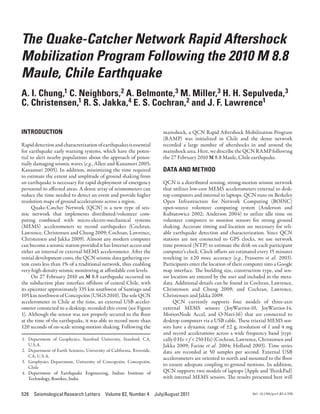
▲ Figure 1. Accelerogram of the M 8.8 mainshock recorded by a station located at the University of Concepción. The dashed line
shows when the initial trigger occurred, soon after the P-wave arrival. Note that the sensor was not fixed to the ground and was resting
on a desk at the time of the mainshock. Around 13 seconds the sensor likely falls off the desk onto the ground.
focus primarily on data recorded by floor-mounted USB accel- the sensors that recorded this event are JW-10 sensors (10-bit
erometers. sensors, 4 mg resolution), but two of the stations are newer
On March 8, 2010, the RAMP deployment of 100 USB QCN sensors (JW-14 and ON-16, 14- and 16-bit sensors with
accelerometers was initiated and a small team of volunteers was 0.24 mg and 0.060 mg resolution, respectively). As expected,
trained on the simple installation procedures. Participants were the higher bit sensors show dramatically lower noise levels.
recruited using an online RAMP sign-up page and, follow- Using manually picked arrivals, we located this event and show
ing local media interviews, over 700 requests for sensors were that the location is similar to U.S. Geological Survey (USGS)
received in roughly one week. Sensors were installed in homes, catalog locations (Figure 3A), suggesting station locations and
police stations, health centers, and other institutions in coor- timing control is accurate enough to test automated event char-
dination with the national emergency authority (ONEMI). acterization algorithms.
To date, QCN has 100 USB sensors and 15 laptop sensors The triggering algorithm is based on the traditional short-
in Chile with sensors deployed mainly in the regions directly term average over long-term average (STA/LTA) method (e.g.,
affected by the mainshock, including a dense cluster of stations Vanderkulk et al. 1965). Here, we use a 0.1-second short-term
near Concepción (Figure 2). These sensors recorded continu- window and a 60-second long-term window. No attempt is
ous waveform data to ensure maximum data recovery and so made to distinguish P and S waves in the initial triggering algo-
event triggering and detection algorithms could be improved rithm, so triggers may represent a mix of phase arrivals. Once
through retrospective testing. The abundance of large after- a trigger is detected at a station, minimal information is trans-
shocks provides a unique opportunity to examine the ability of ferred to a central server and includes station ID, station loca-
this low-cost, distributed sensing network to rapidly detect and tion, sensor type, three-component acceleration at the time of
characterize earthquakes. the trigger, significance, trigger time, and clock offset. In Chile,
approximately half of the stations (48 ± 13) connected to the
RESULTS network each day and sensors are monitored for an average of
about 12.3 ± 2.1 hours per day (Figures 4A, 4B). Using trig-
Using retrospective tests on the continuous data recorded dur- ger data collected between March 1 and June 1, we find that
ing the QCN RAMP, we tested the triggering, event discrimi- the average latencies for trigger information to be transferred
nation, and rapid location and magnitude estimate algorithms. to the central server from Chilean stations is five seconds, with
Figure 3 shows an example of an aftershock recorded by a large more than 90% of the trigger information transmitted in less
number of QCN stations located near Concepción. Most of than eight seconds (Figure 4C).
Seismological Research Letters Volume 82, Number 4 July/August 2011 527

3. (A) Because stations are located in high-noise environments,
60 100 an individual event trigger may represent local noise not related
Mw=4+
Mw=5+
to an earthquake; to distinguish regional ground shaking
Mw=6+
90 events we temporally and spatially correlate incoming triggers.
50 Mw=7+
Mw=8+ 80 We evaluate incoming triggers at 0.2 sec intervals, comparing
each trigger with all other triggers that have occurred in the
Cumulative # QCN Stations
70
40 past 100 seconds. Triggers within 200 km are considered cor-
# Events Per Day
60 related if they occur with a time separation (ΔTij) less than or
equal to the station separation (ΔDij) divided by the slowest
30 # Stations 50
seismic velocity, Vmin plus a small error, ε. This takes the form:
40
20
30
ΔTij ≤ ΔDij ∕ Vmin + ε. (1)
10
20 If the average station to event azimuth is orthogonal to the
10 inter-station azimuth, then ∆Tij should be zero. If the azimuths
are parallel, then ∆Tij should equal the distance divided by the
0 0 velocity. The error, ε, may result from possible inaccuracy intro-
0 10 20 30 40 50
# Days Post Mw=8.8 duced by the trigger algorithm. Once at least five triggers are
correlated, we make an estimate of the earthquake location and
(B) −28°
286° 288° 290°
−28°
magnitude.
The event hypocenter is estimated by performing a three-
dimensional grid search and comparing the predicted and
observed relative arrivals at the stations. The initial event
location is set to the station location with the earliest trigger,
−30° −30°
with the assumption that this sensor is closest to the source.
An initial grid is generated that extends 2° × 2° in latitude and
Station Number longitude with a node every 0.02° and a total depth interval of
100 300 km with nodes every 10 km. The location that minimizes
−32° −32° 90 the L2 misfit between observed and predicted relative travel
80 times is identified as the low-resolution earthquake hypocenter.
70 Using this hypocenter location, we then iterate over a second
60 grid with grid extent and node intervals decreased by an order
−34° −34° 50 of magnitude.
40 Once the location has been estimated, the magnitude is
30 computed using an empirical magnitude distance relation-
20 ship with the acceleration vector magnitude, |a|, similar to the
−36° −36° 10 method of Wu et al. (2003) and Cua and Heaton (2007). This
0 relationship was calibrated using three aftershocks recorded
during the Chile RAMP. The equation is:
−38° −38° N
1
N∑
MI = [ a ln ( b a i ) + c ln ( Di ) + d ] (2)
i =1
286° 288° 290°
▲ Figure 2. A) Number of earthquakes that occurred each day where a = 1.25, b = 1.8, c = 0.8, d = 3.25, and N is the number
versus the number of days after the 27 February 2010 M 8.8 of triggers used. As additional triggers are logged at the server,
Maule mainshock for different magnitude ranges: 4+ (black line), the location and magnitude estimates of the event are updated.
5+ (red line), 6+ (green line), 7+ (blue line), and 8+ (magenta line). We ran a retrospective test of the automated event
Also shown is the cumulative number of QCN stations installed detection and characterization algorithms using aftershocks
(dashed red line). The sensors arrived in Chile one week after the recorded on QCN stations around Concepción March 12–
mainshock and deployment of the sensors began soon afterward. April 3, 2010. Figure 5A shows a map of 23 aftershocks iden-
Almost all of the 100 stations were installed within 10 days after tified by QCN during this 20-day period. The events are all
the deployment began. B) Locations of QCN sensors installed located within the mainshock slip region, which serves as a
after the M 8.8 27 February 2010 Maule mainshock, colored by check on the reliability of the locations. For events detected
station number. Many of the sensors are installed in close prox- by QCN stations and also listed in the National Earthquake
imity to one another and so all sensors may not be visible. Information Center (NEIC) catalog (USGS 2010) we find
528 Seismological Research Letters Volume 82, Number 4 July/August 2011

4. (A) San Juan (C)
Quillota
21
Santiago San Lui
s
Rancagua
24
Chimbarongo
-35° 27
area
Talca
Sensor
100 34
slip
Talcahuano
Los angeles
40
Temuco 50
Neuquen
Distance (km)
44
km
Valdivia
-40° 0 75 150
0 44
-75° -70° -65° 47
(B)
−36° 48
60 70 80 90 100
Con dence 52
−36.5° 54
65
−37° 82
−74° −73.5° −73° −72.5° −72° 0 10 20 30
Time (sec)
▲ Figure 3. A) Map showing the distribution of QCN stations (triangles) colored by installation date, the location of the mainshock epi-
center (red star), and the approximate location of the mainshock rupture plane (gray rectangle). The background color is shaking inten-
sity from the M 8.8 mainshock (e.g., Wald et al. 1999) plotted over topography, with red colors indicating Modified Mercalli Intensity
(MMI) X and green indicating MMI II–IV as illustrated in Figure 6. B) Comparison of USGS/NEIC catalog location and QCN estimated
location for an Mw 5.1 aftershock that occurred on 18 March 2010 at 01:57:33.4 UTC. QCN stations that recorded the event are shown as
blue triangles and the 15-min and 7-day USGS locations are shown by black and red stars, respectively. The QCN-estimated location is
shown by the red circle. Chi-squared statistical confidence is plotted as a color map with 95% and 90% confidence highlighted by the
solid black and dashed black contours, respectively. C) East component time series from the stations to locate the Mw 5.1 aftershock.
Note the reduced noise levels on the new 14-bit and 16-bit sensors shown in purple. P- and S-wave manual picks are shown by the red
and green lines, respectively.
that the magnitude estimates are very similar (Figure 5B). The The average time needed to detect and characterize an
uncertainty of each magnitude estimate is determined through earthquake is 27.4 seconds from the event origin time using the
bootstrap resampling of the trigger information. The average automated scheme described above. The fastest detection occurs
bootstrap uncertainty is approximately 0.45. Updated earth- within 9.4 seconds and the longest delay in detection is 59.2 sec-
quake statistics are generated on a second-by-second basis as onds. Sources of latencies include: source to station wave propa-
new trigger data are archived on the server, with uncertainties gation time, on-site trigger detection, time to transfer trigger
generally decreasing by 10–50% between iterations. information to the server, and computation time. The largest
Seismological Research Letters Volume 82, Number 4 July/August 2011 529

5. (A) (B) (C)
16
Average Uptime (Hours)
Trigger Count (x104)
Number of Stations
60 3
12
40 8 2
20 4 1
0 0 0
0 20 40 60 80 0 20 40 60 80 2 4 6 8 10
Time (Days) Time (Days) Transfer Latency (Sec)
▲ Figure 4. Chile RAMP statistics determined for a three-month period from 1 March to 1 June in 2010. A) Number of stations con-
nected to the network each day. B) Average number of hours each station operated. C) Histogram showing the latencies to transfer the
trigger data from the Chilean stations to the QCN central server in California.
delay in event detection for the Chile aftershock data is the time sensors. The largest delays in event detection were the source-
required for the seismic waves to propagate from the source to station wave propagation times; thus, increasing the density
five or more stations, which is 22 seconds on average. Thus, the of stations would dramatically reduce the detection time.
time required for a station to issue a trigger, send the data to the We expect that the latest generation of sensors will further
server, and compute a location and magnitude is 5.4 seconds, on improve event detection capabilities through increased signal-
average. The delay associated with updating the event character- to-noise ratios resulting in more reliable P-wave detections
istics is also determined by equivalent wave propagation times, for lower magnitude (M < 4.5) events. With little additional
on-site trigger detection, data communication, and server-side computation time we are able to generate maps of measured
computation time, but can happen as quickly as 0.2 seconds or and predicted shaking amplitudes for the region around a
as late as 100 seconds after the event. Again the primary delay moderate to large aftershock. Due to the higher station densi-
factor in updated characteristics is the wave propagation time. ties achievable with low-cost MEMS sensors and distributed
The data collected during the QCN RAMP can also be sensing techniques, it is possible to examine spatial variation
used to provide high-resolution maps of shaking intensity and in ground accelerations at much higher resolution than is
predict shaking intensity using the first few seconds of data practical with traditional instrumentation. Detailed maps of
recorded by the network. Figure 6 illustrates the high similar- shaking intensities could provide critical information to direct
ity between an initial attempt at providing a near real-time emergency responders to regions that experienced the greatest
cyber-enabled shaking intensity map and the USGS ShakeMap accelerations.
(Wald et al. 1999). This map was calculated post-facto, but we Installing 100 sensors in less than two weeks was sur-
account for all latencies including travel-time, data transfer, prisingly attainable. RAMP deployments that utilize MEMS
event characterization, and image publishing. These retrospec- sensor technology may soon be able to install 500 or more
tive simulations typically provide stable shake-maps in less sensors in a populated region immediately following a large
than 30 seconds from the aftershock origin time. The shake- earthquake. Furthermore, with the arrival of the more sensi-
maps are also rapidly updated as new trigger data arrive. tive 14-bit, 16-bit, and 24-bit accelerometers, it will be possible
to record more aftershocks at greater resolution. The greatest
DISCUSSION delay in QCN’s RAMP installation was in making appropriate
local contacts for obtaining unrestricted access to the rupture
Due to the portability of the USB MEMS accelerometers and zone. Through the combination of cyber, social, and seismic
simple installation procedure, a dense real-time network of networking, QCN is rapidly overcoming this hurdle.
strong-motion seismic stations was installed rapidly following Having a very dense network of hundreds, or even thou-
the 27 February 2010 M 8.8 Maule, Chile earthquake. Most sands, of low-cost sensors in a region of high seismicity will
of the 100 stations were installed within 10 days of the RAMP provide higher resolution estimates of small-scale lateral varia-
initiation, and we were thus able to record many of the initial, tions in amplification effects than previously possible. This will
significant aftershocks. Rapid event detection and character- enable us to better understand on what scales heterogeneities
ization is very important for directing emergency response and cause amplification, focusing, and defocusing (e.g., Gao et al.
is critical for the future development of earthquake advanced 1996). QCN strong-motion data can also provide dense obser-
alert systems (e.g., Allen et al. 2009; Kanamori 2005). vations around a large earthquake, resulting in higher-resolu-
As shown, we can rapidly estimate aftershock locations tion slip models and enhanced understanding of rupture prop-
and magnitudes using data from the QCN strong-motion erties (e.g., Dreger et al. 2005; Jakka et al. 2010).
530 Seismological Research Letters Volume 82, Number 4 July/August 2011

6. (A) 285 286 287 288 289 290 (B) 7
-35 -35 Mb(QCN)=0.96Mb(NEIC)
6
-36 -36
Mb (NEIC)
5
-37 -37 Co-detected
4
-38 -38
QCN -Only
-39 -39 3
3 4 5 6 7
285 286 287 288 289 290 Mb (QCN)
▲ Figure 5. A) Aftershock locations (red circles) determined by a retrospective, automated event location scheme that uses trigger
information from QCN stations (blue triangles) located near Concepción. Star shows the mainshock epicenter and rectangle repre-
sents the approximate mainshock slip plane. B) Event magnitudes between March 12 and April 30, 2010 for events co-detected by NEIC
and QCN (black squares) and events detected only by QCN (gray diamonds). The black line is a fit to the co-detected events showing
reasonable agreement between QCN-estimated magnitudes compared to NEIC catalog magnitudes.
(A) Curico (B) Curico
–35° –35°
-35°
Talca Talca
–35.5° –35.5°
-35.5°
Linares Linares
–36° Parral
–36° Parral
San Carlos San Carlos
–36.5° –36.5°
Talcahuano Talcahuano
–37° Coronel
–37° Coronel
Arauco Arauco
Los angeles Los angeles
–37.5° km –37.5° km
Lebu Mulchen Lebu Mulchen
0 50 0 50
–74° –73° –72° –74° –73° –72°
PERCEIVED
SHAKING Not felt Weak Light Moderate Strong Very strong Severe Violent Extreme
POTENTIAL none none none Very light Light Moderate Moderate/Heavy Heavy Very Heavy
DAMAGE
PEAK ACC.(%g) <.17 .17–1.
4 1.4–3.
9 3.9–9.
2 9.2–18 18–34 34–65 65–124 >124
PEAK VEL.(cm/s) <0.1 0.1–1. 1.1–3.4
1 3.4–8.
1 8.1–16 16–31 31–60 60–116 >116
INSTRUMENTAL
INTENSITY I II–III IV V VI VII VIII IX X+
▲ Figure 6. Comparison between (A) USGS ShakeMap (from USGS 2010) and (B) QCN cyber-enabled hazard map for the 16 March 2010
Mw 5.5 earthquake located offshore of Concepción.
Seismological Research Letters Volume 82, Number 4 July/August 2011 531

7. ACKNOWLEDGMENTS Frassetto, A., T. J. Owens, and P. Crotwell (2003). Evaluating the net-
work time protocol (NTP) for timing in the South Carolina Earth
Physics Project (SCEPP). Seismological Research Letters 74, 649–
This research was funded by NSF RAPID Award EAR 1035919 652.
and NSF grant EAR-0952376. The authors would also like to Gao, S., H. Liu, P. M. Davis, and L. Knopoff (1996). Localized ampli-
thank geology and geophysics students from the University of fication of seismic waves and correlation with damage due to the
Concepción for their invaluable assistance with deploying the Northridge earthquake: Evidence for focusing in Santa Monica.
sensors. Bulletin of the Seismological Society of America 86, S209–S230.
Holland, J. (2003). Earthquake data recorded by the MEMS accelerom-
eter. Seismological Research Letters 74, 20–26.
REFERENCES Jakka, R. S., E. S. Cochran, and J. F. Lawrence (2010). Earthquake source
characterization by the isochrone back projection method using
Allen, R. M., and H. Kanamori (2003). The potential for earthquake near-source ground motions. Geophysical Journal International
early warning in Southern California. Science 300, 786–789. doi:10.111/j.1365-246X.2010.04670.x.
Allen, R. M., H. Brown, M. Hellweg, O. Khainovski, P. Lombard, D. Kanamori, H. (2005). Real-time seismology and earthquake damage
Neuhauser (2009). Real-time earthquake detection and hazard mitigation. Annual Review of Earth and Planetary Science 33,
assessment by ElarmS across California. Geophysical Research 195–214.
Letters 36, L00B08, doi:10.1029/2008GL036766. USGS (2010). ShakeMap us2010txak: Offshore Bio-Bio, Chile
Anderson, D. P. (2004). BOINC: A system for public-resource comput- ht tp ://ear thquake.usgs.gov/ear thquakes/shakemap/global/
ing and storage. Proceedings of the Fifth IEEE/ACM International shake/2010txai/
Workshop on Grid Computing, November 8, 2004, Pittsburgh, Vanderkulk, W., F. Rosen, and S. Lorenz (1965). Large Aperture Seismic
USA, 4−10: http://www.computer.org/portal/web/csdl/abs/pro- Array Signal Processing Study. IBM Final Report, AROA Contract
ceedings/grid/2004/2256/00/2256toc.htm SD-296.
Anderson, D. P., and J. Kubiatowicz (2002). The world-wide computer. Wald, D. J., V. Quitoriano, T. H. Heaton, H. Kanamori, C. W. Scrivner,
Scientific American 286, 40–47. and C. B. Worden (1999). TriNet “ShakeMaps”: rapid generation of
Cochran, E. S., J. F. Lawrence, C. Christensen, A. I. Chung (2009). A peak ground motion and intensity maps for earthquakes in south-
novel strong-motion seismic network for community participation ern California (1999). TriNet “ShakeMaps”: Rapid generation of
in earthquake monitoring. Institute of Electrical and Electronics peak ground motion and intensity maps for earthquakes in south-
Engineers Instruments and Measures 12, 8–15. ern California. Earthquake Spectra 15, 537–555.
Cochran, E. S., J. F. Lawrence, C. Christensen, and R. Jakka (2009). The Wu, Y.-M., T.-l. Teng, T.-C. Shin, and N.-C. Hsiao (2003). Relationship
Quake-Catcher Network: Citizen science expanding seismic hori- between peak ground acceleration, peak ground velocity, and inten-
zons. Seismological Research Letters 80, 26–30. sity in Taiwan. Bulletin of the Seismological Society of America 93,
Cua, G., and T. H. Heaton (2007). The Virtual Seismologist (VS) 386–396.
method: A Bayesian approach to earthquake early warning. In
Earthquake Early Warning Systems, ed. P. Gasparini, G. Manfredi, Department of Geophysics
and J. Zschau, 97–132. Berlin & New York: Springer.
Dreger, D. S., L. Gee, P. Lombard, M. H. Murray, and Barbara Stanford University
Romanowicz (2005). Rapid finite-source analysis and near-fault 397 Panama Mall
strong ground motions: Application to the 2003 Mw 6.5 San Stanford, California 94305 U.S.A.
Simeon and 2004 Mw 6.0 Parkfield earthquakes. Seismological aichung@stanford.edu
Research Letters 76, 40–48. (A. I. C.)
Farine, M., N. Thorburn, and D. Mougenot (2004). General applica-
tion of MEMS sensors for land seismic acquisition, is it time? The
Leading Edge 23, 246–250.
532 Seismological Research Letters Volume 82, Number 4 July/August 2011