1. MS Excel 2010 Features
Formatting Cells
Cells are the small rectangular boxes that make up the spreadsheet. All the information
entered into an Excel spreadsheet is entered into cells.
The cell width and height will usually need to be adjusted to view all the information
entered into a cell.
To adjust the cell width, move the mouse pointer in between two cell columns in the
column header. Hold down the left mouse button and drag the
mouse left to shorten the width or right to expand the width. Notice
that all cells within the column are automatically adjusted.
Adjust the cell height using the same method. Move the mouse cursor
between two rows, hold down the left mouse button and move the mouse up to
decrease the height and down to increase the height.
Before you begin entering data into a spreadsheet, you may already know the width and
height you want your cells to have. In this case, you can adjust all the widths and heights
by doing the following:
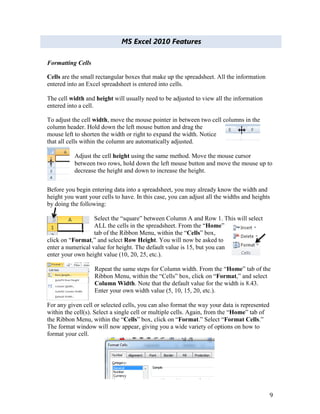
Select the “square” between Column A and Row 1. This will select
ALL the cells in the spreadsheet. From the “Home”
tab of the Ribbon Menu, within the “Cells” box,
click on “Format,” and select Row Height. You will now be asked to
enter a numerical value for height. The default value is 15, but you can
enter your own height value (10, 20, 25, etc.).
Repeat the same steps for Column width. From the “Home” tab of the
Ribbon Menu, within the “Cells” box, click on “Format,” and select
Column Width. Note that the default value for the width is 8.43.
Enter your own width value (5, 10, 15, 20, etc.).
For any given cell or selected cells, you can also format the way your data is represented
within the cell(s). Select a single cell or multiple cells. Again, from the “Home” tab of
the Ribbon Menu, within the “Cells” box, click on “Format.” Select “Format Cells.”
The format window will now appear, giving you a wide variety of options on how to
format your cell.
9

2. Number – This allows you to choose how to represent the numbers that are entered into a
cell (number, currency, time, etc.).
Alignment – This determines how the data will be aligned within the cell (left-side,
centered, or right-side).
Font – Select the type of font to be used within the cells.
Border – This option lets you choose what type of border, if any, you would like around
the cells or some of the cells.
Fill – This allows you to change the background color of the cell.
Protection – This option allows you to “lock” cell information so that other users cannot
make changes.
Typing in Cells
Click on a cell to begin typing in it. It is that easy! When you are finished typing in the
cell, press the Enter key and you will be taken to the next cell down. You can then begin
typing in that cell. You can easily navigate around the cells using your arrow keys.
Keep in mind that the Formatting toolbar in Microsoft Excel 2010 is exactly the same as
the one used for Microsoft Word 2010. The biggest difference between the two programs
is that, in Excel, the format is set for each individual cell. So if you change the font and
applied the bold option in cell C5, then this format will only be applied to cell C5. All
remaining cells will remain in default mode until they have been changed.
Sometimes you may only wish to adjust the format of one particular cell. In this case,
simply select the cell by clicking the mouse on it and make any necessary adjustments to
the font, size, style, and alignment. Those changes will not carry over when you begin
typing in a new cell.
Other times, you may wish to adjust the text format of a group of cells, entire rows, or
entire columns.
In Excel, you can choose groups of cells in rectangular units—all the cells you select
must form a rectangle of some kind. To select a group of cells, begin by clicking on the
cell that would be in the upper-left hand corner of your rectangle. Hold down the Shift
key on your keyboard and use the arrows (←, →, ↑, ↓) on the keyboard to expand the
selection of cells, or click and drag your mouse.
Once the group of cells has been selected, you can make adjustments to the font, size,
style, and alignment and they will be applied to all selected cells.
To select an entire row, click on the
Row Number with your mouse—note
10

3. how the entire row becomes highlighted. All formatting changes will now be applied to
the whole row.
To select an entire column, click on the Column Number with your mouse—
again, the entire column will become highlighted. All formatting changes will
be applied to the whole column.
Inserting Rows and Columns
When you are working on a spreadsheet, you may realize that you left out a row or
column of data and need to add it in.
To insert a row, click on the row below where you want your new row to be (remember
to click on the row number to highlight the entire row). From the “Home” tab, within the
“Cells” box, click “Insert.” Select “Insert Sheet
Rows.” A new row will automatically be inserted and
the row numbers automatically adjusted.
To insert a column, click on the column to the right of
where you want your new column to be (remember to
click on the column letter to highlight the entire
column). From the “Home” tab, within the “Cells” box,
click “Insert.” Select “Insert Sheet Columns.” A new
column will automatically be inserted and the column
letters automatically adjusted.
Sorting Data
Once you have created your spreadsheet and entered in some data, you may want to
organize the data in a certain way. This could be alphabetically, numerically, or another
way. Let’s look at the following spreadsheet as an example.
This information can be sorted by check number, date, alphabetically by description, or
using any of the other columns.
11

4. First, select all the cells that represent the data to be sorted, including the header
descriptions (Check No., Date, Description, etc.). Then, select the first cell in Row 1
(Check No.) Click and drag to select all the cells that you want to sort.
Using the mouse, select Sort & Filter from the Editing panel. Select Custom Sort…
The following window should appear:
Select the column you wish to sort by. Do you want to sort by alphabetical order, reverse
alphabetical order, date, or amount? When you press “OK,” your spreadsheet will be sorted in
the order that you specified.
Advanced Spreadsheet Modification
Once you have created a basic spreadsheet there are numerous things you can do to make
working with you data easier. Some of these elements are hiding, freezing and splitting rows.
You can also sort and filter data, these features are quite helpful when working with a large
amount of data.
Hide or Display Rows and Columns
You can hide a row or column by using the Hide command or when you change its row
height or column width to 0 (zero). You can display either again by using the Unhide
command. You can either unhide specific rows and columns, or you can unhide all hidden
rows and columns at the same time. The first row or column of the worksheet is tricky to
unhide, but it can be done.
Hide Rows or Columns
1. Select the rows or columns that you want to hide.
2. On the Home tab, in the Cells group, click Format.
3. Under Visibility, point to Hide & Unhide, and then click Hide
Rows or Hide Columns.
NOTE: You can also right-click a row or column (or a
selection of multiple rows or columns), and then click
Hide.
Unhide Rows or Columns

5. 1. Select the rows, columns or entire sheet to unhide.
2. On the Home tab, in the Cells group, click Format.
3. Under Visibility, point to Hide & Unhide, and then click Unhide
Rows or Unhide Columns.
TIP You can also right-click the selection of visible rows and
columns surrounding the hidden rows and columns, and then click Unhide.