Workshop on Introduction to Eviews-26th of February 2014

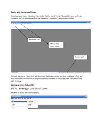
1. Dealing with the start up of Eviews
If you have your Eviews in desktop, then, double click the icon of Eviews (*Eviews 6) to open up Eviews.
Otherwise, you can select Eviews from the Start Menu. (Start Menu - All programs –Eviews)
Command Line
Menus-Drop
down menus
Current path
The main features of Eviews deals with Command Line(for generating functions, conditional effects and
etc), drop down menus (selection of option to perform different actions) and current path (refers to the
path directory).
Opening up Eviews file (workfile)
Click File – direct to Open – point to Eviews workfile
Workfile of choice refers to macro data

2. Select macro data.wf1 and click on Open
The opening of workfile is shown as below:-
Range
Sample
Variables

3. Examination on single mode of variable
Select gdp from the list and double click on it. It will show the spreadsheet view of gdp.
Click on the View button and it will reveal some options such as spreadsheet, graph, descriptive
statistics and tests, one way tabulation and etc. Select Graph and click on it. Then, it will show up the
dialog box on graph options.
Select Distribution in the specific box and Select Histogram. It will show up histogram of gdp.

4. Click View and then select Graph. Once again, it will reveal the dialog box of graph options.
Select Distribution from the specific box and select Histogram. Then, click options and it will direct to
the dialog box on Distribution Plot Customize.

5. Click Add. It will reveal the dialog box of add and it will show different types of elements such as
Histogram, Histogram Polygon, histogram Edge Polygon, Average Shifted Histogram, Kernel Density,
and Theoretical density.
Select Theoretical density.

6. It will reveal a dialog box on Distribution Plot Customize and theoretical distribution has been added to
added elements.
Click ok and it will reveal the dialog box of graph options. It can be noticed that distribution has been
changed to custom.

7. Click ok and it will reveal the histogram with normal curve.
Click View and select Descriptive Statistics & Tests. Direct to Histogram and Stats. It will reveal
histogram and stats table
Click the histogram and press Ctrl + C to copy the graph. A dialog box on graph metafile will appear as
below:-

8. Click ok and paste it in word file. It will appear as below:-
Now, it’s time to get back to the workfile. To identify the descriptive statistics of three variables (dmr,
gdp and invest), highlight all the three variables by holding Ctrl. It will be as below:-

9. Right click on it and select open as a group.
Then, the spreadsheet view on the selected variables will be as below:-

10. Click View and select Descriptive Statistics, direct to Common Sample.
The descriptive statistics of the selected variables will be as below:-

11. Press Ctrl + A to highlight the portions of descriptive statistics of the variables. It will be as below:-
Press Ctrl + C to copy the table and a dialog box will appear as below:-
Click ok and paste it in Word file. It will be shown as below:-

12. Now, it’s time to get back to workfile. Click View and select Graph.
A dialog box will appear as below:-

13. Then, select Line& Symbol in the specific box and select Multiple graphs. It can be seen as below

14. Click ok and the multiple graphs will appear as below
Close it and highlight two variables(gdp and invest). The illustration is as below:-

15. Right click on it and select Open as a group. Spreadsheet view on the selected variables will be shown
as below:-
Click View and select Graph. It is shown as below:-
A dialog box will appear as below:-

16. Select Scatter in the specific box and click ok. Scatter plot between GDP and INVEST can be seen as
below:-
Click View and select Graph. A dialog box on graph options will appear again

17. Select Scatter and choose Regression line. Scatter plot with regression line between gdp and invest will
be as below:-

18. Click View and select Graph. A dialog box on graph options will appear again
Select Quantile-Quantile in the specific table and select Theoretical. Then, click Ok. The graphical
illustrations of QQ plot are shown as below:-
Close/Save it and then Click Quick and select Group Statistics and then, direct to Covariances

19. A dialog box will appear as below:-
Click ok and the results will shown as below:-

20. Click Quick and select Group Statistics and direct to Correlations
A dialog box will appear
The results of correlations will be as below:-
Linear Regression
Click Quick and select Estimate Equation

21. A Dialog box will appear
It is a must to fill up dependent variable(gdp) followed by c (constant), and independent
variables(unemp and invest).

22. Click ok and the results will appear as below:-
Click View and select Representations. The representations will be as below:-

23. Click View and select Actual, Fitted Residuals and then point to Actual, Fitted Residual Table
It will be shown as below:-

24. Click View and select Actual, Fitted Residual and then direct to Actual ,Fitted Residual Graph
The illustration of graph will be as below:-

25. Click View and select Actual, Fitted Residuals and then direct to Residual Graph
The illustration of graph will be as below:-

26. Click View and select Residual tests and direct to Histogram-Normality Test
The results will be as below:-