SlideShare une entreprise Scribd logo
1  sur  59
2
of
60
Towards the Ideal Line
We can only do a discrete approximation
Illuminate pixels as close to the true path as
possible, consider bi-level display only
– Pixels are either lit or not lit
3
of
60
What is an ideal line
Must appear straight and continuous
– Only possible axis-aligned and 45o
lines
Must interpolate both defining end points
Must have uniform density and intensity
– Consistent within a line and over all lines
– What about antialiasing?
Must be efficient, drawn quickly
– Lots of them are required!!!
UPES-Graphics
4
of
60
Simple Line
Based on slope-intercept
algorithm from algebra:
y = mx + b
Simple approach:
increment x, solve for y
Floating point arithmetic
required
5
of
60
LINE-DRAWING
ALGORITHMS
6
of
60
Does it Work?
It seems to work okay for
lines with a slope of 1 or
less,
but doesn’t work well for
lines with slope greater than
1 – lines become more
discontinuous in appearance
and we must add more than
1 pixel per column to make it
work.
Solution? - use symmetry.
7
of
60
Modify algorithm per octant
OR, increment along x-axis if dy<dx
else increment along y-axis
8
of
60
DDA algorithm
DDA = Digital Differential Analyser
– finite differences
Treat line as parametric equation in t :
)()(
)()(
121
121
yytyty
xxtxtx
−+=
−+=),(
),(
22
11
yx
yxStart point -
End point -
9
of
60
DDA Algorithm
Start at t = 0
At each step, increment t by dt
Choose appropriate value for dt
Ensure no pixels are missed:
– Implies: and
Set dt to maximum of dx and dy
)()(
)()(
121
121
yytyty
xxtxtx
−+=
−+=
dt
dy
yy
dt
dx
xx
oldnew
oldnew
+=
+=
1<
dt
dx
1<
dt
dy
10
of
60
DDA Algorithm
The digital differential analyzer (DDA)
myyxm kk +=⇒=∆⇒≤< +110.10.0 myyxm kk +=⇒=∆⇒≤< +110.10.0
m
xxym kk
1
10.1 1 +=⇒=∆⇒< +
m
xxym kk
1
10.1 1 −=⇒=∆⇒>− +
myyxm kk −=⇒=∆⇒−≥> +110.10.0
Equations are based on the assumption that lines are to be processed from
the left endpoint to the right endpoint.
11
of
60
#include 'device. h"
void lineDDA (int xa, int ya, int xb, int yb)
{ int dx = xb - xa, dy = yb - ya, steps, k;
float xIncrement, yIncrement, x = xa, y = ya;
if ( abs(dx) > abs(dy) ) steps = abs (dx) ;
else steps = abs dy);
xIncrement = dx / (float) steps;
yIncrement = dy / (float) steps;
setpixel (ROUNDlxl, ROUND(y) ) :
for (k=O; k<steps; k++) {
x += xIncrment;
y += yIncrement;
setpixel (ROUND(x), ROUND(y));
DDA Algorithm
12
of
60
DDA algorithm
line(int x1, int y1, int x2, int y2)
{
float x,y;
int dx = x2-x1, dy = y2-y1;
int n = max(abs(dx),abs(dy));
float dt = n, dxdt = dx/dt, dydt = dy/dt;
x = x1;
y = y1;
while( n-- ) {
point(round(x),round(y));
x += dxdt;
y += dydt;
}
}
n - range of t.
UPES-Graphics
13
of
60
DDA algorithm
Still need a lot of floating point arithmetic.
– 2 ‘round’s and 2 adds per pixel.
Is there a simpler way ?
Can we use only integer arithmetic ?
– Easier to implement in hardware.
UPES-Graphics
14
of
60
Raster Scan System Random Scan System
Resolution It has poor or less Resolution because picture definition is
stored as a intensity value.
It has High Resolution because it stores picture definition as a
set of line commands.
Electron-Beam Electron Beam is directed from top to bottom and one row at a
time on screen, but electron beam is directed to whole screen.
Electron Beam is directed to only that part of screen where
picture is required to be drawn, one line at a time so also
called Vector Display.
Cost It is less expensive than Random Scan System. It is Costlier than Raster Scan System.
Refresh Rate Refresh rate is 60 to 80 frame per second. Refresh Rate depends on the number of lines to be displayed
i.e 30 to 60 times per second.
Picture Definition It Stores picture definition in Refresh Bufferalso
called Frame Buffer.
It Stores picture definition as a set of line
commandscalled Refresh Display File.
Line Drawing Zig – Zag line is produced because plotted value are discrete. Smooth line is produced because directly the line path is
followed by electron beam .
Realism in display It contains shadow, advance shading and hidden surface
technique so gives the realistic display of scenes.
It does not contain shadow and hidden surface technique so it
can not give realistic display of scenes.
Image Drawing It uses Pixels along scan lines for drawing an image. It is designed for line drawing applications and uses various
mathematical function to draw.
Difference Between Raster Scan ystem and Random Scan System.
15
of
60
The Bresenham Line Algorithm
The Bresenham algorithm is
another incremental scan
conversion algorithm
The big advantage of this
algorithm is that it uses only
integer calculations
Jack Bresenham
worked for 27 years at
IBM before entering
academia. Bresenham
developed his famous
algorithms at IBM in
the early 1960s
16
of
60
The Big Idea
Move across the x axis in unit intervals and
at each step choose between two different y
coordinates
2 3 4 5
2
4
3
5
For example, from
position (2, 3) we
have to choose
between (3, 3) and
(3, 4)
We would like the
point that is closer to
the original line
(xk, yk)
(xk+1, yk)
(xk+1, yk+1)
17
of
60
The y coordinate on the mathematical line at
xk+1 is:
Deriving The Bresenham Line Algorithm
At sample position xk+1
the vertical separations
from the mathematical
line are labelled dupper
and dlower
bxmy k ++= )1(
y
yk
yk+1
xk+1
dlower
dupper
18
of
60
So, dupper and dlower are given as follows:
and:
We can use these to make a simple decision
about which pixel is closer to the mathematical
line
Deriving The Bresenham Line Algorithm
(cont…)
klower yyd −=
kk ybxm −++= )1(
yyd kupper −+= )1(
bxmy kk −+−+= )1(1
19
of
60
This simple decision is based on the difference
between the two pixel positions:
Let’s substitute m with ∆y/∆x where ∆x and
∆y are the differences between the end-points:
Deriving The Bresenham Line Algorithm
(cont…)
122)1(2 −+−+=− byxmdd kkupperlower
)122)1(2()( −+−+
∆
∆
∆=−∆ byx
x
y
xddx kkupperlower
)12(222 −∆+∆+⋅∆−⋅∆= bxyyxxy kk
cyxxy kk +⋅∆−⋅∆= 22
20
of
60
So, a decision parameter pk for the kth step
along a line is given by:
The sign of the decision parameter pk is the
same as that of dlower – dupper
If pk is negative, then we choose the lower
pixel, otherwise we choose the upper pixel
Deriving The Bresenham Line Algorithm
(cont…)
cyxxy
ddxp
kk
upperlowerk
+⋅∆−⋅∆=
−∆=
22
)(
21
of
60
Remember coordinate changes occur along
the x axis in unit steps so we can do
everything with integer calculations
At step k+1 the decision parameter is given
as:
Subtracting pk from this we get:
Deriving The Bresenham Line Algorithm
(cont…)
cyxxyp kkk +⋅∆−⋅∆= +++ 111 22
)(2)(2 111 kkkkkk yyxxxypp −∆−−∆=− +++
22
of
60
But, xk+1 is the same as xk+1 so:
where yk+1 - yk is either 0 or 1 depending on
the sign of pk
The first decision parameter p0 is evaluated
at (x0, y0) is given as:
Deriving The Bresenham Line Algorithm
(cont…)
)(22 11 kkkk yyxypp −∆−∆+= ++
xyp ∆−∆= 20
23
of
60
The Bresenham Line Algorithm
BRESENHAM’S LINE DRAWING ALGORITHM
(for |m| < 1.0)
1. Input the two line end-points, storing the left end-point
in (x0, y0)
2. Plot the point (x0, y0)
3. Calculate the constants Δx, Δy, 2Δy, and (2Δy - 2Δx)
and get the first value for the decision parameter as:
4. At each xk along the line, starting at k = 0, perform the
following test. If pk < 0, the next point to plot is
(xk+1, yk) and:
xyp ∆−∆= 20
ypp kk ∆+=+ 21
24
of
60
The Bresenham Line Algorithm (cont…)
ACHTUNG! The algorithm and derivation
above assumes slopes are less than 1. for
other slopes we need to adjust the algorithm
slightly
Otherwise, the next point to plot is (xk+1, yk+1) and:
5. Repeat step 4 (Δx – 1) times
xypp kk ∆−∆+=+ 221
25
of
60
Bresenham Example
Let’s have a go at this
Let’s plot the line from (20, 10) to (30, 18)
First off calculate all of the constants:
– Δx: 10
– Δy: 8
– 2Δy: 16
– 2Δy - 2Δx: -4
Calculate the initial decision parameter p0:
– p0 = 2Δy – Δx = 6
26
of
60
Bresenham Example (cont…)
17
16
15
14
13
12
11
10
18
292726252423222120 28 30
k Pk
(xk+1,yk+1)
0
1
2
3
4
5
6
7
8
9
P0
27
of
60
Bresenham Exercise
Go through the steps of the Bresenham line
drawing algorithm for a line going from
(21,12) to (29,16)
28
of
60
Bresenham Exercise (cont…)
17
16
15
14
13
12
11
10
18
292726252423222120 28 30
k pk
(xk+1,yk+1)
0
1
2
3
4
5
6
7
8
29
of
60
Bresenham Line Algorithm Summary
The Bresenham line algorithm has the
following advantages:
– An fast incremental algorithm
– Uses only integer calculations
Comparing this to the DDA algorithm, DDA
has the following problems:
– Accumulation of round-off errors can make
the pixelated line drift away from what was
intended
– The rounding operations and floating point
arithmetic involved are time consuming
30
of
60
A Simple Circle Drawing Algorithm
The equation for a circle is:
where r is the radius of the circle
So, we can write a simple circle drawing
algorithm by solving the equation for y at
unit x intervals using:
222
ryx =+
22
xry −±=
31
of
60
A Simple Circle Drawing Algorithm
(cont…)
20020 22
0 ≈−=y
20120 22
1 ≈−=y
20220 22
2 ≈−=y
61920 22
19 ≈−=y
02020 22
20 ≈−=y
32
of
60
A Simple Circle Drawing Algorithm
(cont…)
However, unsurprisingly this is not a brilliant
solution!
Firstly, the resulting circle has large gaps
where the slope approaches the vertical
Secondly, the calculations are not very
efficient
– The square (multiply) operations
– The square root operation – try really hard to
avoid these!
We need a more efficient, more accurate
solution
33
of
60
Eight-Way Symmetry
The first thing we can notice to make our circle
drawing algorithm more efficient is that circles
centred at (0, 0) have eight-way symmetry
(x, y)
(y, x)
(y, -x)
(x, -y)(-x, -y)
(-y, -x)
(-y, x)
(-x, y)
2
R
34
of
60
Mid-Point Circle Algorithm
Similarly to the case with lines,
there is an incremental
algorithm for drawing circles –
the mid-point circle algorithm
In the mid-point circle algorithm
we use eight-way symmetry so
only ever calculate the points
for the top right eighth of a
circle, and then use symmetry
to get the rest of the points
The mid-point circle
algorithm was
developed by Jack
Bresenham, who we
heard about earlier.
Bresenham’s patent
for the algorithm can
be viewed here.
35
of
60
Mid-Point Circle Algorithm (cont…)
(xk+1, yk)
(xk+1, yk-1)
(xk, yk)
Assume that we have
just plotted point (xk, yk)
The next point is a
choice between (xk+1, yk)
and (xk+1, yk-1)
We would like to choose
the point that is nearest to
the actual circle
So how do we make this choice?
36
of
60
Mid-Point Circle Algorithm (cont…)
the equation of the circle slightly to give us:
The equation evaluates as follows:
By evaluating this function at the midpoint
between the candidate pixels we can make
our decision
222
),( ryxyxfcirc −+=





>
=
<
,0
,0
,0
),( yxfcirc
boundarycircletheinsideis),(if yx
boundarycircleon theis),(if yx
boundarycircletheoutsideis),(if yx
37
of
60
Mid-Point Circle Algorithm (cont…)
Assuming we have just plotted the pixel at
(xk,yk) so we need to choose between (xk+1,yk)
and (xk+1,yk-1)
Our decision variable can be defined as:
If pk < 0 the midpoint is inside the circle and
and the pixel at yk is closer to the circle
Otherwise the midpoint is outside and yk-1 is
222
)
2
1()1(
)
2
1,1(
ryx
yxfp
kk
kkcirck
−−++=
−+=
38
of
60
Mid-Point Circle Algorithm (cont…)
To ensure things are as efficient as possible
we can do all of our calculations
incrementally
First consider:
or:
where yk+1 is either yk or yk-1 depending on
the sign of p
( )
( ) 2
2
1
2
111
2
1]1)1[(
2
1,1
ryx
yxfp
kk
kkcirck
−−+++=
−+=
+
+++
1)()()1(2 1
22
11 +−−−+++= +++ kkkkkkk yyyyxpp
39
of
60
Mid-Point Circle Algorithm (cont…)
The first decision variable is given as:
Then if pk < 0 then the next decision variable
is given as:
If pk > 0 then the decision variable is:
r
rr
rfp circ
−=
−−+=
−=
4
5
)
2
1(1
)
2
1,1(
22
0
12 11 ++= ++ kkk xpp
1212 11 +−++= ++ kkkk yxpp
40
of
60
The Mid-Point Circle Algorithm
MID-POINT CIRCLE ALGORITHM
• Input radius r and circle centre (xc, yc), then set the
coordinates for the first point on the circumference of a
circle centred on the origin as:
• Calculate the initial value of the decision parameter as:
• Starting with k = 0 at each position xk, perform the
following test. If pk< 0, the next point along the circle
centred on (0, 0) is (xk+1, yk) and:
),0(),( 00 ryx =
rp −=
4
5
0
12 11 ++= ++ kkk xpp
41
of
60
The Mid-Point Circle Algorithm (cont…)
Otherwise the next point along the circle is (xk+1, yk-1)
and:
Where 2xk+1=2xk+2and 2yk+1=2yk-2
4. Determine symmetry points in the other seven octants
5. Move each calculated pixel position (x, y) onto the
circular path centred at (xc, yc) to plot the coordinate
values:
6. Repeat steps 3 to 5 until x >= y
111 212 +++ −++= kkkk yxpp
cxxx += cyyy +=
42
of
60
Mid-Point Circle Algorithm Example
To see the mid-point circle algorithm in
action lets use it to draw a circle centred at
(0,0) with radius 10
43
of
60
Mid-Point Circle Algorithm Example
(cont…)
9
7
6
5
4
3
2
1
0
8
976543210 8 10
10
k pk
(xk+1,yk+1) 2xk+1 2yk+1
0
1
2
3
4
5
6
44
of
60
Mid-Point Circle Algorithm Exercise
Use the mid-point circle algorithm to draw
the circle centred at (0,0) with radius 15
45
of
60
Mid-Point Circle Algorithm Example
(cont…)
k pk (xk+1,yk+1) 2xk+1
2yk+1
0
1
2
3
4
5
6
7
8
9
10
11
12
9
7
6
5
4
3
2
1
0
8
976543210 8 10
10
131211 14
15
13
12
14
11
16
1516
46
of
60
Mid-Point Circle Algorithm Summary
The key insights in the mid-point circle
algorithm are:
– Eight-way symmetry can hugely reduce the
work in drawing a circle
– Moving in unit steps along the x axis at each
point along the circle’s edge we need to
choose between two possible y coordinates
47
of
60
Filling Polygons
So we can figure out how to draw lines and
circles
How do we go about drawing polygons?
We use an incremental algorithm known as
the scan-line algorithm
48
of
60
Scan-Line Polygon Fill Algorithm
2
4
6
8
10 Scan Line
0
2 4 6 8 10 12 14 16
49
of
60
Scan-Line Polygon Fill Algorithm
The basic scan-line algorithm is as follows:
– Find the intersections of the scan line with all
edges of the polygon
– Sort the intersections by increasing x
coordinate
– Fill in all pixels between pairs of intersections
that lie interior to the polygon
50
of
60
Scan-Line Polygon Fill Algorithm
(cont…)
51
of
60
Line Drawing Summary
Over the last couple of lectures we have
looked at the idea of scan converting lines
The key thing to remember is this has to be
FAST
For lines we have either DDA or Bresenham
For circles the mid-point algorithm
52
of
60
Anti-Aliasing
53
of
60
Summary Of Drawing Algorithms
54
of
60
Mid-Point Circle Algorithm (cont…)
6
2 3 41
5
4
3
55
of
60
Mid-Point Circle Algorithm (cont…)
M
6
2 3 41
5
4
3
56
of
60
Mid-Point Circle Algorithm (cont…)
M
6
2 3 41
5
4
3
57
of
60
Blank Grid
58
of
60
Blank Grid
59
of
60
Blank Grid
9
7
6
5
4
3
2
1
0
8
976543210 8 10
10
60
of
60
Blank Grid

Contenu connexe

Tendances

Bresenham circlesandpolygons
Bresenham circlesandpolygonsBresenham circlesandpolygons
Bresenham circlesandpolygons
aa11bb11
 
Bresenham's line algo.
Bresenham's line algo.Bresenham's line algo.
Bresenham's line algo.
Mohd Arif
 
Lines and curves algorithms
Lines and curves algorithmsLines and curves algorithms
Lines and curves algorithms
Mohammad Sadiq
 
Graphics6 bresenham circlesandpolygons
Graphics6 bresenham circlesandpolygonsGraphics6 bresenham circlesandpolygons
Graphics6 bresenham circlesandpolygons
Ketan Jani
 
Line drawing algo.
Line drawing algo.Line drawing algo.
Line drawing algo.
Mohd Arif
 
Line drawing algorithm and antialiasing techniques
Line drawing algorithm and antialiasing techniquesLine drawing algorithm and antialiasing techniques
Line drawing algorithm and antialiasing techniques
Ankit Garg
 
Midpoint circle algo
Midpoint circle algoMidpoint circle algo
Midpoint circle algo
Mohd Arif
 

Tendances (20)

Computer Graphics - Bresenham's line drawing algorithm & Mid Point Circle alg...
Computer Graphics - Bresenham's line drawing algorithm & Mid Point Circle alg...Computer Graphics - Bresenham's line drawing algorithm & Mid Point Circle alg...
Computer Graphics - Bresenham's line drawing algorithm & Mid Point Circle alg...
 
Lab lecture 2 bresenham
Lab lecture 2 bresenhamLab lecture 2 bresenham
Lab lecture 2 bresenham
 
bresenham circles and polygons in computer graphics(Computer graphics tutorials)
bresenham circles and polygons in computer graphics(Computer graphics tutorials)bresenham circles and polygons in computer graphics(Computer graphics tutorials)
bresenham circles and polygons in computer graphics(Computer graphics tutorials)
 
Cs580
Cs580Cs580
Cs580
 
Bresenham circlesandpolygons
Bresenham circlesandpolygonsBresenham circlesandpolygons
Bresenham circlesandpolygons
 
Bresenham's line algo.
Bresenham's line algo.Bresenham's line algo.
Bresenham's line algo.
 
Lines and curves algorithms
Lines and curves algorithmsLines and curves algorithms
Lines and curves algorithms
 
Bresenhamcircle derivation
Bresenhamcircle derivationBresenhamcircle derivation
Bresenhamcircle derivation
 
Dda line-algorithm
Dda line-algorithmDda line-algorithm
Dda line-algorithm
 
Chapter 3 Output Primitives
Chapter 3 Output PrimitivesChapter 3 Output Primitives
Chapter 3 Output Primitives
 
Graphics6 bresenham circlesandpolygons
Graphics6 bresenham circlesandpolygonsGraphics6 bresenham circlesandpolygons
Graphics6 bresenham circlesandpolygons
 
DDA algorithm
DDA algorithmDDA algorithm
DDA algorithm
 
Dda algorithm
Dda algorithmDda algorithm
Dda algorithm
 
Line drawing algo.
Line drawing algo.Line drawing algo.
Line drawing algo.
 
Bresenham's line algorithm
Bresenham's line algorithmBresenham's line algorithm
Bresenham's line algorithm
 
Dda algo notes
Dda algo notesDda algo notes
Dda algo notes
 
Line drawing algorithm and antialiasing techniques
Line drawing algorithm and antialiasing techniquesLine drawing algorithm and antialiasing techniques
Line drawing algorithm and antialiasing techniques
 
Computer graphics - bresenham line drawing algorithm
Computer graphics - bresenham line drawing algorithmComputer graphics - bresenham line drawing algorithm
Computer graphics - bresenham line drawing algorithm
 
Midpoint circle algo
Midpoint circle algoMidpoint circle algo
Midpoint circle algo
 
BRESENHAM’S LINE DRAWING ALGORITHM
BRESENHAM’S  LINE DRAWING ALGORITHMBRESENHAM’S  LINE DRAWING ALGORITHM
BRESENHAM’S LINE DRAWING ALGORITHM
 

En vedette

Lecture filling algorithms
Lecture  filling algorithmsLecture  filling algorithms
Lecture filling algorithms
avelraj
 
Visible surface detection in computer graphic
Visible surface detection in computer graphicVisible surface detection in computer graphic
Visible surface detection in computer graphic
anku2266
 
hidden surface elimination using z buffer algorithm
hidden surface elimination using z buffer algorithmhidden surface elimination using z buffer algorithm
hidden surface elimination using z buffer algorithm
rajivagarwal23dei
 

En vedette (9)

Lect14 lines+circles
Lect14 lines+circlesLect14 lines+circles
Lect14 lines+circles
 
Hidden Surface Removal using Z-buffer
Hidden Surface Removal using Z-bufferHidden Surface Removal using Z-buffer
Hidden Surface Removal using Z-buffer
 
Lecture filling algorithms
Lecture  filling algorithmsLecture  filling algorithms
Lecture filling algorithms
 
visible surface detection
visible surface detectionvisible surface detection
visible surface detection
 
Visible surface detection in computer graphic
Visible surface detection in computer graphicVisible surface detection in computer graphic
Visible surface detection in computer graphic
 
Computer Graphics: Visible surface detection methods
Computer Graphics: Visible surface detection methodsComputer Graphics: Visible surface detection methods
Computer Graphics: Visible surface detection methods
 
Digital Differential Analyzer Line Drawing Algorithm
Digital Differential Analyzer Line Drawing AlgorithmDigital Differential Analyzer Line Drawing Algorithm
Digital Differential Analyzer Line Drawing Algorithm
 
Output primitives in Computer Graphics
Output primitives in Computer GraphicsOutput primitives in Computer Graphics
Output primitives in Computer Graphics
 
hidden surface elimination using z buffer algorithm
hidden surface elimination using z buffer algorithmhidden surface elimination using z buffer algorithm
hidden surface elimination using z buffer algorithm
 

Similaire à Bresenham circles and polygons derication

Output Primitives in Computer Graphics and Multimedia
Output Primitives in Computer Graphics and MultimediaOutput Primitives in Computer Graphics and Multimedia
Output Primitives in Computer Graphics and Multimedia
saranyan75
 
Computer Graphics and Multimedia Output primitives
Computer Graphics and Multimedia Output primitivesComputer Graphics and Multimedia Output primitives
Computer Graphics and Multimedia Output primitives
saranyan75
 

Similaire à Bresenham circles and polygons derication (20)

Computer graphics notes
Computer graphics notesComputer graphics notes
Computer graphics notes
 
Unit 2
Unit 2Unit 2
Unit 2
 
Unit-2 raster scan graphics,line,circle and polygon algorithms
Unit-2 raster scan graphics,line,circle and polygon algorithmsUnit-2 raster scan graphics,line,circle and polygon algorithms
Unit-2 raster scan graphics,line,circle and polygon algorithms
 
Computer graphics 2
Computer graphics 2Computer graphics 2
Computer graphics 2
 
Computer graphics notes watermark
Computer graphics notes watermarkComputer graphics notes watermark
Computer graphics notes watermark
 
raster algorithm.pdf
raster algorithm.pdfraster algorithm.pdf
raster algorithm.pdf
 
Computer Graphics Unit 1
Computer Graphics Unit 1Computer Graphics Unit 1
Computer Graphics Unit 1
 
Computer Graphics Unit 2
Computer Graphics Unit 2Computer Graphics Unit 2
Computer Graphics Unit 2
 
1536 graphics &amp; graphical programming
1536 graphics &amp; graphical  programming1536 graphics &amp; graphical  programming
1536 graphics &amp; graphical programming
 
Output Primitives in Computer Graphics and Multimedia
Output Primitives in Computer Graphics and MultimediaOutput Primitives in Computer Graphics and Multimedia
Output Primitives in Computer Graphics and Multimedia
 
Computer Graphics and Multimedia Output primitives
Computer Graphics and Multimedia Output primitivesComputer Graphics and Multimedia Output primitives
Computer Graphics and Multimedia Output primitives
 
03.Scan Conversion.ppt
03.Scan Conversion.ppt03.Scan Conversion.ppt
03.Scan Conversion.ppt
 
Computer graphics lab manual
Computer graphics lab manualComputer graphics lab manual
Computer graphics lab manual
 
Line Drawing Algorithms - Computer Graphics - Notes
Line Drawing Algorithms - Computer Graphics - NotesLine Drawing Algorithms - Computer Graphics - Notes
Line Drawing Algorithms - Computer Graphics - Notes
 
module 1.pdf
module 1.pdfmodule 1.pdf
module 1.pdf
 
cgrchapter2version-1-200729063505 (1).pdf
cgrchapter2version-1-200729063505 (1).pdfcgrchapter2version-1-200729063505 (1).pdf
cgrchapter2version-1-200729063505 (1).pdf
 
Computer graphics notes 2 tutorials duniya
Computer graphics notes 2   tutorials duniyaComputer graphics notes 2   tutorials duniya
Computer graphics notes 2 tutorials duniya
 
Lecture-4-Scan_Conversion_Bresenhams_Algorithm.ppt
Lecture-4-Scan_Conversion_Bresenhams_Algorithm.pptLecture-4-Scan_Conversion_Bresenhams_Algorithm.ppt
Lecture-4-Scan_Conversion_Bresenhams_Algorithm.ppt
 
Rasterization.pptx
Rasterization.pptxRasterization.pptx
Rasterization.pptx
 
lecture 1.pptx
lecture 1.pptxlecture 1.pptx
lecture 1.pptx
 

Plus de Kumar (20)

Graphics devices
Graphics devicesGraphics devices
Graphics devices
 
Fill area algorithms
Fill area algorithmsFill area algorithms
Fill area algorithms
 
region-filling
region-fillingregion-filling
region-filling
 
Introductionto xslt
Introductionto xsltIntroductionto xslt
Introductionto xslt
 
Extracting data from xml
Extracting data from xmlExtracting data from xml
Extracting data from xml
 
Xml basics
Xml basicsXml basics
Xml basics
 
XML Schema
XML SchemaXML Schema
XML Schema
 
Publishing xml
Publishing xmlPublishing xml
Publishing xml
 
DTD
DTDDTD
DTD
 
Applying xml
Applying xmlApplying xml
Applying xml
 
Introduction to XML
Introduction to XMLIntroduction to XML
Introduction to XML
 
How to deploy a j2ee application
How to deploy a j2ee applicationHow to deploy a j2ee application
How to deploy a j2ee application
 
JNDI, JMS, JPA, XML
JNDI, JMS, JPA, XMLJNDI, JMS, JPA, XML
JNDI, JMS, JPA, XML
 
EJB Fundmentals
EJB FundmentalsEJB Fundmentals
EJB Fundmentals
 
JSP and struts programming
JSP and struts programmingJSP and struts programming
JSP and struts programming
 
java servlet and servlet programming
java servlet and servlet programmingjava servlet and servlet programming
java servlet and servlet programming
 
Introduction to JDBC and JDBC Drivers
Introduction to JDBC and JDBC DriversIntroduction to JDBC and JDBC Drivers
Introduction to JDBC and JDBC Drivers
 
Introduction to J2EE
Introduction to J2EEIntroduction to J2EE
Introduction to J2EE
 
Android tutorial (2)
Android tutorial (2)Android tutorial (2)
Android tutorial (2)
 
Android structure
Android structureAndroid structure
Android structure
 

Dernier

1029-Danh muc Sach Giao Khoa khoi 6.pdf
1029-Danh muc Sach Giao Khoa khoi  6.pdf1029-Danh muc Sach Giao Khoa khoi  6.pdf
1029-Danh muc Sach Giao Khoa khoi 6.pdf
QucHHunhnh
 

Dernier (20)

Dyslexia AI Workshop for Slideshare.pptx
Dyslexia AI Workshop for Slideshare.pptxDyslexia AI Workshop for Slideshare.pptx
Dyslexia AI Workshop for Slideshare.pptx
 
Explore beautiful and ugly buildings. Mathematics helps us create beautiful d...
Explore beautiful and ugly buildings. Mathematics helps us create beautiful d...Explore beautiful and ugly buildings. Mathematics helps us create beautiful d...
Explore beautiful and ugly buildings. Mathematics helps us create beautiful d...
 
Unit-V; Pricing (Pharma Marketing Management).pptx
Unit-V; Pricing (Pharma Marketing Management).pptxUnit-V; Pricing (Pharma Marketing Management).pptx
Unit-V; Pricing (Pharma Marketing Management).pptx
 
Mehran University Newsletter Vol-X, Issue-I, 2024
Mehran University Newsletter Vol-X, Issue-I, 2024Mehran University Newsletter Vol-X, Issue-I, 2024
Mehran University Newsletter Vol-X, Issue-I, 2024
 
TỔNG ÔN TẬP THI VÀO LỚP 10 MÔN TIẾNG ANH NĂM HỌC 2023 - 2024 CÓ ĐÁP ÁN (NGỮ Â...
TỔNG ÔN TẬP THI VÀO LỚP 10 MÔN TIẾNG ANH NĂM HỌC 2023 - 2024 CÓ ĐÁP ÁN (NGỮ Â...TỔNG ÔN TẬP THI VÀO LỚP 10 MÔN TIẾNG ANH NĂM HỌC 2023 - 2024 CÓ ĐÁP ÁN (NGỮ Â...
TỔNG ÔN TẬP THI VÀO LỚP 10 MÔN TIẾNG ANH NĂM HỌC 2023 - 2024 CÓ ĐÁP ÁN (NGỮ Â...
 
Mixin Classes in Odoo 17 How to Extend Models Using Mixin Classes
Mixin Classes in Odoo 17  How to Extend Models Using Mixin ClassesMixin Classes in Odoo 17  How to Extend Models Using Mixin Classes
Mixin Classes in Odoo 17 How to Extend Models Using Mixin Classes
 
Spatium Project Simulation student brief
Spatium Project Simulation student briefSpatium Project Simulation student brief
Spatium Project Simulation student brief
 
Micro-Scholarship, What it is, How can it help me.pdf
Micro-Scholarship, What it is, How can it help me.pdfMicro-Scholarship, What it is, How can it help me.pdf
Micro-Scholarship, What it is, How can it help me.pdf
 
How to Create and Manage Wizard in Odoo 17
How to Create and Manage Wizard in Odoo 17How to Create and Manage Wizard in Odoo 17
How to Create and Manage Wizard in Odoo 17
 
Unit-IV- Pharma. Marketing Channels.pptx
Unit-IV- Pharma. Marketing Channels.pptxUnit-IV- Pharma. Marketing Channels.pptx
Unit-IV- Pharma. Marketing Channels.pptx
 
ICT Role in 21st Century Education & its Challenges.pptx
ICT Role in 21st Century Education & its Challenges.pptxICT Role in 21st Century Education & its Challenges.pptx
ICT Role in 21st Century Education & its Challenges.pptx
 
psychiatric nursing HISTORY COLLECTION .docx
psychiatric  nursing HISTORY  COLLECTION  .docxpsychiatric  nursing HISTORY  COLLECTION  .docx
psychiatric nursing HISTORY COLLECTION .docx
 
ICT role in 21st century education and it's challenges.
ICT role in 21st century education and it's challenges.ICT role in 21st century education and it's challenges.
ICT role in 21st century education and it's challenges.
 
General Principles of Intellectual Property: Concepts of Intellectual Proper...
General Principles of Intellectual Property: Concepts of Intellectual  Proper...General Principles of Intellectual Property: Concepts of Intellectual  Proper...
General Principles of Intellectual Property: Concepts of Intellectual Proper...
 
Food safety_Challenges food safety laboratories_.pdf
Food safety_Challenges food safety laboratories_.pdfFood safety_Challenges food safety laboratories_.pdf
Food safety_Challenges food safety laboratories_.pdf
 
Basic Civil Engineering first year Notes- Chapter 4 Building.pptx
Basic Civil Engineering first year Notes- Chapter 4 Building.pptxBasic Civil Engineering first year Notes- Chapter 4 Building.pptx
Basic Civil Engineering first year Notes- Chapter 4 Building.pptx
 
SKILL OF INTRODUCING THE LESSON MICRO SKILLS.pptx
SKILL OF INTRODUCING THE LESSON MICRO SKILLS.pptxSKILL OF INTRODUCING THE LESSON MICRO SKILLS.pptx
SKILL OF INTRODUCING THE LESSON MICRO SKILLS.pptx
 
1029-Danh muc Sach Giao Khoa khoi 6.pdf
1029-Danh muc Sach Giao Khoa khoi  6.pdf1029-Danh muc Sach Giao Khoa khoi  6.pdf
1029-Danh muc Sach Giao Khoa khoi 6.pdf
 
Holdier Curriculum Vitae (April 2024).pdf
Holdier Curriculum Vitae (April 2024).pdfHoldier Curriculum Vitae (April 2024).pdf
Holdier Curriculum Vitae (April 2024).pdf
 
Unit-IV; Professional Sales Representative (PSR).pptx
Unit-IV; Professional Sales Representative (PSR).pptxUnit-IV; Professional Sales Representative (PSR).pptx
Unit-IV; Professional Sales Representative (PSR).pptx
 

Bresenham circles and polygons derication

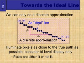
  • 1. 2 of 60 Towards the Ideal Line We can only do a discrete approximation Illuminate pixels as close to the true path as possible, consider bi-level display only – Pixels are either lit or not lit
  • 2. 3 of 60 What is an ideal line Must appear straight and continuous – Only possible axis-aligned and 45o lines Must interpolate both defining end points Must have uniform density and intensity – Consistent within a line and over all lines – What about antialiasing? Must be efficient, drawn quickly – Lots of them are required!!! UPES-Graphics
  • 3. 4 of 60 Simple Line Based on slope-intercept algorithm from algebra: y = mx + b Simple approach: increment x, solve for y Floating point arithmetic required
  • 5. 6 of 60 Does it Work? It seems to work okay for lines with a slope of 1 or less, but doesn’t work well for lines with slope greater than 1 – lines become more discontinuous in appearance and we must add more than 1 pixel per column to make it work. Solution? - use symmetry.
  • 6. 7 of 60 Modify algorithm per octant OR, increment along x-axis if dy<dx else increment along y-axis
  • 7. 8 of 60 DDA algorithm DDA = Digital Differential Analyser – finite differences Treat line as parametric equation in t : )()( )()( 121 121 yytyty xxtxtx −+= −+=),( ),( 22 11 yx yxStart point - End point -
  • 8. 9 of 60 DDA Algorithm Start at t = 0 At each step, increment t by dt Choose appropriate value for dt Ensure no pixels are missed: – Implies: and Set dt to maximum of dx and dy )()( )()( 121 121 yytyty xxtxtx −+= −+= dt dy yy dt dx xx oldnew oldnew += += 1< dt dx 1< dt dy
  • 9. 10 of 60 DDA Algorithm The digital differential analyzer (DDA) myyxm kk +=⇒=∆⇒≤< +110.10.0 myyxm kk +=⇒=∆⇒≤< +110.10.0 m xxym kk 1 10.1 1 +=⇒=∆⇒< + m xxym kk 1 10.1 1 −=⇒=∆⇒>− + myyxm kk −=⇒=∆⇒−≥> +110.10.0 Equations are based on the assumption that lines are to be processed from the left endpoint to the right endpoint.
  • 10. 11 of 60 #include 'device. h" void lineDDA (int xa, int ya, int xb, int yb) { int dx = xb - xa, dy = yb - ya, steps, k; float xIncrement, yIncrement, x = xa, y = ya; if ( abs(dx) > abs(dy) ) steps = abs (dx) ; else steps = abs dy); xIncrement = dx / (float) steps; yIncrement = dy / (float) steps; setpixel (ROUNDlxl, ROUND(y) ) : for (k=O; k<steps; k++) { x += xIncrment; y += yIncrement; setpixel (ROUND(x), ROUND(y)); DDA Algorithm
  • 11. 12 of 60 DDA algorithm line(int x1, int y1, int x2, int y2) { float x,y; int dx = x2-x1, dy = y2-y1; int n = max(abs(dx),abs(dy)); float dt = n, dxdt = dx/dt, dydt = dy/dt; x = x1; y = y1; while( n-- ) { point(round(x),round(y)); x += dxdt; y += dydt; } } n - range of t. UPES-Graphics
  • 12. 13 of 60 DDA algorithm Still need a lot of floating point arithmetic. – 2 ‘round’s and 2 adds per pixel. Is there a simpler way ? Can we use only integer arithmetic ? – Easier to implement in hardware. UPES-Graphics
  • 13. 14 of 60 Raster Scan System Random Scan System Resolution It has poor or less Resolution because picture definition is stored as a intensity value. It has High Resolution because it stores picture definition as a set of line commands. Electron-Beam Electron Beam is directed from top to bottom and one row at a time on screen, but electron beam is directed to whole screen. Electron Beam is directed to only that part of screen where picture is required to be drawn, one line at a time so also called Vector Display. Cost It is less expensive than Random Scan System. It is Costlier than Raster Scan System. Refresh Rate Refresh rate is 60 to 80 frame per second. Refresh Rate depends on the number of lines to be displayed i.e 30 to 60 times per second. Picture Definition It Stores picture definition in Refresh Bufferalso called Frame Buffer. It Stores picture definition as a set of line commandscalled Refresh Display File. Line Drawing Zig – Zag line is produced because plotted value are discrete. Smooth line is produced because directly the line path is followed by electron beam . Realism in display It contains shadow, advance shading and hidden surface technique so gives the realistic display of scenes. It does not contain shadow and hidden surface technique so it can not give realistic display of scenes. Image Drawing It uses Pixels along scan lines for drawing an image. It is designed for line drawing applications and uses various mathematical function to draw. Difference Between Raster Scan ystem and Random Scan System.
  • 14. 15 of 60 The Bresenham Line Algorithm The Bresenham algorithm is another incremental scan conversion algorithm The big advantage of this algorithm is that it uses only integer calculations Jack Bresenham worked for 27 years at IBM before entering academia. Bresenham developed his famous algorithms at IBM in the early 1960s
  • 15. 16 of 60 The Big Idea Move across the x axis in unit intervals and at each step choose between two different y coordinates 2 3 4 5 2 4 3 5 For example, from position (2, 3) we have to choose between (3, 3) and (3, 4) We would like the point that is closer to the original line (xk, yk) (xk+1, yk) (xk+1, yk+1)
  • 16. 17 of 60 The y coordinate on the mathematical line at xk+1 is: Deriving The Bresenham Line Algorithm At sample position xk+1 the vertical separations from the mathematical line are labelled dupper and dlower bxmy k ++= )1( y yk yk+1 xk+1 dlower dupper
  • 17. 18 of 60 So, dupper and dlower are given as follows: and: We can use these to make a simple decision about which pixel is closer to the mathematical line Deriving The Bresenham Line Algorithm (cont…) klower yyd −= kk ybxm −++= )1( yyd kupper −+= )1( bxmy kk −+−+= )1(1
  • 18. 19 of 60 This simple decision is based on the difference between the two pixel positions: Let’s substitute m with ∆y/∆x where ∆x and ∆y are the differences between the end-points: Deriving The Bresenham Line Algorithm (cont…) 122)1(2 −+−+=− byxmdd kkupperlower )122)1(2()( −+−+ ∆ ∆ ∆=−∆ byx x y xddx kkupperlower )12(222 −∆+∆+⋅∆−⋅∆= bxyyxxy kk cyxxy kk +⋅∆−⋅∆= 22
  • 19. 20 of 60 So, a decision parameter pk for the kth step along a line is given by: The sign of the decision parameter pk is the same as that of dlower – dupper If pk is negative, then we choose the lower pixel, otherwise we choose the upper pixel Deriving The Bresenham Line Algorithm (cont…) cyxxy ddxp kk upperlowerk +⋅∆−⋅∆= −∆= 22 )(
  • 20. 21 of 60 Remember coordinate changes occur along the x axis in unit steps so we can do everything with integer calculations At step k+1 the decision parameter is given as: Subtracting pk from this we get: Deriving The Bresenham Line Algorithm (cont…) cyxxyp kkk +⋅∆−⋅∆= +++ 111 22 )(2)(2 111 kkkkkk yyxxxypp −∆−−∆=− +++
  • 21. 22 of 60 But, xk+1 is the same as xk+1 so: where yk+1 - yk is either 0 or 1 depending on the sign of pk The first decision parameter p0 is evaluated at (x0, y0) is given as: Deriving The Bresenham Line Algorithm (cont…) )(22 11 kkkk yyxypp −∆−∆+= ++ xyp ∆−∆= 20
  • 22. 23 of 60 The Bresenham Line Algorithm BRESENHAM’S LINE DRAWING ALGORITHM (for |m| < 1.0) 1. Input the two line end-points, storing the left end-point in (x0, y0) 2. Plot the point (x0, y0) 3. Calculate the constants Δx, Δy, 2Δy, and (2Δy - 2Δx) and get the first value for the decision parameter as: 4. At each xk along the line, starting at k = 0, perform the following test. If pk < 0, the next point to plot is (xk+1, yk) and: xyp ∆−∆= 20 ypp kk ∆+=+ 21
  • 23. 24 of 60 The Bresenham Line Algorithm (cont…) ACHTUNG! The algorithm and derivation above assumes slopes are less than 1. for other slopes we need to adjust the algorithm slightly Otherwise, the next point to plot is (xk+1, yk+1) and: 5. Repeat step 4 (Δx – 1) times xypp kk ∆−∆+=+ 221
  • 24. 25 of 60 Bresenham Example Let’s have a go at this Let’s plot the line from (20, 10) to (30, 18) First off calculate all of the constants: – Δx: 10 – Δy: 8 – 2Δy: 16 – 2Δy - 2Δx: -4 Calculate the initial decision parameter p0: – p0 = 2Δy – Δx = 6
  • 26. 27 of 60 Bresenham Exercise Go through the steps of the Bresenham line drawing algorithm for a line going from (21,12) to (29,16)
  • 28. 29 of 60 Bresenham Line Algorithm Summary The Bresenham line algorithm has the following advantages: – An fast incremental algorithm – Uses only integer calculations Comparing this to the DDA algorithm, DDA has the following problems: – Accumulation of round-off errors can make the pixelated line drift away from what was intended – The rounding operations and floating point arithmetic involved are time consuming
  • 29. 30 of 60 A Simple Circle Drawing Algorithm The equation for a circle is: where r is the radius of the circle So, we can write a simple circle drawing algorithm by solving the equation for y at unit x intervals using: 222 ryx =+ 22 xry −±=
  • 30. 31 of 60 A Simple Circle Drawing Algorithm (cont…) 20020 22 0 ≈−=y 20120 22 1 ≈−=y 20220 22 2 ≈−=y 61920 22 19 ≈−=y 02020 22 20 ≈−=y
  • 31. 32 of 60 A Simple Circle Drawing Algorithm (cont…) However, unsurprisingly this is not a brilliant solution! Firstly, the resulting circle has large gaps where the slope approaches the vertical Secondly, the calculations are not very efficient – The square (multiply) operations – The square root operation – try really hard to avoid these! We need a more efficient, more accurate solution
  • 32. 33 of 60 Eight-Way Symmetry The first thing we can notice to make our circle drawing algorithm more efficient is that circles centred at (0, 0) have eight-way symmetry (x, y) (y, x) (y, -x) (x, -y)(-x, -y) (-y, -x) (-y, x) (-x, y) 2 R
  • 33. 34 of 60 Mid-Point Circle Algorithm Similarly to the case with lines, there is an incremental algorithm for drawing circles – the mid-point circle algorithm In the mid-point circle algorithm we use eight-way symmetry so only ever calculate the points for the top right eighth of a circle, and then use symmetry to get the rest of the points The mid-point circle algorithm was developed by Jack Bresenham, who we heard about earlier. Bresenham’s patent for the algorithm can be viewed here.
  • 34. 35 of 60 Mid-Point Circle Algorithm (cont…) (xk+1, yk) (xk+1, yk-1) (xk, yk) Assume that we have just plotted point (xk, yk) The next point is a choice between (xk+1, yk) and (xk+1, yk-1) We would like to choose the point that is nearest to the actual circle So how do we make this choice?
  • 35. 36 of 60 Mid-Point Circle Algorithm (cont…) the equation of the circle slightly to give us: The equation evaluates as follows: By evaluating this function at the midpoint between the candidate pixels we can make our decision 222 ),( ryxyxfcirc −+=      > = < ,0 ,0 ,0 ),( yxfcirc boundarycircletheinsideis),(if yx boundarycircleon theis),(if yx boundarycircletheoutsideis),(if yx
  • 36. 37 of 60 Mid-Point Circle Algorithm (cont…) Assuming we have just plotted the pixel at (xk,yk) so we need to choose between (xk+1,yk) and (xk+1,yk-1) Our decision variable can be defined as: If pk < 0 the midpoint is inside the circle and and the pixel at yk is closer to the circle Otherwise the midpoint is outside and yk-1 is 222 ) 2 1()1( ) 2 1,1( ryx yxfp kk kkcirck −−++= −+=
  • 37. 38 of 60 Mid-Point Circle Algorithm (cont…) To ensure things are as efficient as possible we can do all of our calculations incrementally First consider: or: where yk+1 is either yk or yk-1 depending on the sign of p ( ) ( ) 2 2 1 2 111 2 1]1)1[( 2 1,1 ryx yxfp kk kkcirck −−+++= −+= + +++ 1)()()1(2 1 22 11 +−−−+++= +++ kkkkkkk yyyyxpp
  • 38. 39 of 60 Mid-Point Circle Algorithm (cont…) The first decision variable is given as: Then if pk < 0 then the next decision variable is given as: If pk > 0 then the decision variable is: r rr rfp circ −= −−+= −= 4 5 ) 2 1(1 ) 2 1,1( 22 0 12 11 ++= ++ kkk xpp 1212 11 +−++= ++ kkkk yxpp
  • 39. 40 of 60 The Mid-Point Circle Algorithm MID-POINT CIRCLE ALGORITHM • Input radius r and circle centre (xc, yc), then set the coordinates for the first point on the circumference of a circle centred on the origin as: • Calculate the initial value of the decision parameter as: • Starting with k = 0 at each position xk, perform the following test. If pk< 0, the next point along the circle centred on (0, 0) is (xk+1, yk) and: ),0(),( 00 ryx = rp −= 4 5 0 12 11 ++= ++ kkk xpp
  • 40. 41 of 60 The Mid-Point Circle Algorithm (cont…) Otherwise the next point along the circle is (xk+1, yk-1) and: Where 2xk+1=2xk+2and 2yk+1=2yk-2 4. Determine symmetry points in the other seven octants 5. Move each calculated pixel position (x, y) onto the circular path centred at (xc, yc) to plot the coordinate values: 6. Repeat steps 3 to 5 until x >= y 111 212 +++ −++= kkkk yxpp cxxx += cyyy +=
  • 41. 42 of 60 Mid-Point Circle Algorithm Example To see the mid-point circle algorithm in action lets use it to draw a circle centred at (0,0) with radius 10
  • 42. 43 of 60 Mid-Point Circle Algorithm Example (cont…) 9 7 6 5 4 3 2 1 0 8 976543210 8 10 10 k pk (xk+1,yk+1) 2xk+1 2yk+1 0 1 2 3 4 5 6
  • 43. 44 of 60 Mid-Point Circle Algorithm Exercise Use the mid-point circle algorithm to draw the circle centred at (0,0) with radius 15
  • 44. 45 of 60 Mid-Point Circle Algorithm Example (cont…) k pk (xk+1,yk+1) 2xk+1 2yk+1 0 1 2 3 4 5 6 7 8 9 10 11 12 9 7 6 5 4 3 2 1 0 8 976543210 8 10 10 131211 14 15 13 12 14 11 16 1516
  • 45. 46 of 60 Mid-Point Circle Algorithm Summary The key insights in the mid-point circle algorithm are: – Eight-way symmetry can hugely reduce the work in drawing a circle – Moving in unit steps along the x axis at each point along the circle’s edge we need to choose between two possible y coordinates
  • 46. 47 of 60 Filling Polygons So we can figure out how to draw lines and circles How do we go about drawing polygons? We use an incremental algorithm known as the scan-line algorithm
  • 47. 48 of 60 Scan-Line Polygon Fill Algorithm 2 4 6 8 10 Scan Line 0 2 4 6 8 10 12 14 16
  • 48. 49 of 60 Scan-Line Polygon Fill Algorithm The basic scan-line algorithm is as follows: – Find the intersections of the scan line with all edges of the polygon – Sort the intersections by increasing x coordinate – Fill in all pixels between pairs of intersections that lie interior to the polygon
  • 49. 50 of 60 Scan-Line Polygon Fill Algorithm (cont…)
  • 50. 51 of 60 Line Drawing Summary Over the last couple of lectures we have looked at the idea of scan converting lines The key thing to remember is this has to be FAST For lines we have either DDA or Bresenham For circles the mid-point algorithm
  • 53. 54 of 60 Mid-Point Circle Algorithm (cont…) 6 2 3 41 5 4 3
  • 54. 55 of 60 Mid-Point Circle Algorithm (cont…) M 6 2 3 41 5 4 3
  • 55. 56 of 60 Mid-Point Circle Algorithm (cont…) M 6 2 3 41 5 4 3

Notes de l'éditeur

  1. Important algorithm.