1. Chapter 25 Page 1
Inventory Theory
Inventories are materials stored, waiting for processing, or experiencing processing.
They are ubiquitous throughout all sectors of the economy. Observation of almost any
company balance sheet, for example, reveals that a significant portion of its assets
comprises inventories of raw materials, components and subassemblies within the
production process, and finished goods. Most managers don't like inventories because
they are like money placed in a drawer, assets tied up in investments that are not
producing any return and, in fact, incurring a borrowing cost. They also incur costs for
the care of the stored material and are subject to spoilage and obsolescence. In the last
two decades their have been a spate of programs developed by industry, all aimed at
reducing inventory levels and increasing efficiency on the shop floor. Some of the most
popular are conwip, kanban, just-in-time manufacturing, lean manufacturing, and flexible
manufacturing.
Nevertheless, in spite of the bad features associated with inventories, they do have
positive purposes. Raw material inventories provide a stable source of input required for
production. A large inventory requires fewer replenishments and may reduce ordering
costs because of economies of scale. In-process inventories reduce the impacts of the
variability of the production rates in a plant and protect against failures in the processes.
Final goods inventories provide for better customer service. The variety and easy
availability of the product is an important marketing consideration. There are other kinds
of inventories, including spare parts inventories for maintenance and excess capacity built
into facilities to take advantage of the economies of scale of construction.
Because of their practical and economic importance, the subject of inventory
control is a major consideration in many situations. Questions must be constantly
answered as to when and how much raw material should be ordered, when a production
order should be released to the plant, what level of safety stock should be maintained at a
retail outlet, or how in-process inventory is to be maintained in a production process.
These questions are amenable to quantitative analysis with the help of inventory theory.
25.1 Inventory Models
In this chapter, we will consider several types of models starting with the deterministic
case in the next section. Even though many features of an inventory system involve
uncertainty of some kind, it is common to assume much simpler deterministic models for
which solutions are found using calculus. Deterministic models also provide a base on
which to incorporate assumptions concerning uncertainty. Section 25.3 adds a stochastic
dimension to the model with random product demand. Section 25.4 begins discussion of
stochastic inventory systems with the single period stochastic model. The model has
applications for products for which the ordering process is nonrepeating. The remainder
of the chapter addresses models with an infinite time horizon and several assumptions
5/30/02

2. 2 Inventory Theory
regarding the costs of operation. Sections 25.5 and 25.6 derive optimal solutions for the
(s, S) policy under a variety of conditions. This policy places an order up to level S when
the inventory level falls to the reorder point s. Section 25.7 extends these results to the
(R, S) policy. In this case, the inventory is observed periodically (with a time interval R),
and is replenished to level S.
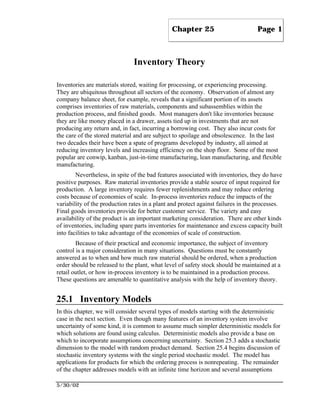
Flow, Inventory and Time
An inventory is represented in the simple diagram of Fig. 1. Items flow
into the system, remain for a time and then flow out. Inventories occur
whenever the time an individual enters is different than when it leaves.
During the intervening interval the item is part of the inventory.
Flow In Inventory Level Flow Out
(Residence Time)
Figure 1. A system component with inventory
For example, say the box in Fig. 1 represents a manufacturing
process that takes a fixed amount of time. A product entering the box at
one moment leaves the box one hour later. Products arrive at a rate of 100
per hour. Clearly, if we look in the box, we will find some number of
items. That number is the inventory level. The relation between flow,
time and inventory level that is basic to all systems is
Inventory level = (Flow rate )(Residence time) (1)
where the flow rate is expressed in the same time units as the residence
time. For the example, we have
Inventory Level = (100 products/hour )(1 hour) = 100 products.
When the factors in Eq. (1) are not constant in time, we typically use their
mean values.
Whenever two of the factors in the above expression are given, the
third is easily computed. Consider a queueing system for which customers
are observed to arrive at an average rate of 10 per hour. When the
customer finds the servers busy, he or she must wait. Customers in the
system, either waiting or be served, are the inventory for this system.
Using a sampling procedure we determine that the average number of
customers in the inventory is 5. We ask, how long on the average is each
customer in the system? Using the relation between the flow, time and

3. Inventory Models 3
inventory, we determine the answer as 0.5 hours. As we saw in the
Chapter 16, Queueing Models, Eq (1) is called Little's Law.
The relation between time and inventory is significant, because
very often reducing the throughput time for a system is just as important
as reducing the inventory level. Since they are proportional, changing one
factor inevitably changes the other.
The Inventory Level
The inventory level depends on the relative rates of flow in and out of the
system. Define y(t) as the rate of input flow at time t and Y(t) the
cumulative flow into the system. Define z(t) as the rate of output flow at
time t and Z(t) as the cumulative flow out of the system. The inventory
level, I(t) is the cumulative input less the cumulative output.
t t
I(t) = Y(t) – Z(t) = ⌠y(x)dx - ⌠z(x)dx
⌡ ⌡ (2)
0 0
Figure 2 represents the inventory for a system when the rates vary with
time.
Inventory Level
0
0 Time
Figure 2. Inventory fluctuations as a function of time
The figure might represent a raw material inventory. The flow out
of inventory is a relatively continuous activity where individual items are
placed into the production system for processing. To replenish the
inventory, an order is placed to a supplier. After some delay time, called
the lead time, the raw material is delivered in a lot of a specified amount.
At the moment of delivery, the rate of input is infinite and at other times it
is zero. Whenever the instantaneous rates of input and output to a
component are not the same, the inventory level changes. When the input
rate is higher, inventory grows; when output rate is higher, inventory
declines.
Usually the inventory level remains positive. This corresponds to
the presence of on hand inventory. In cases where the cumulative output

4. 4 Inventory Theory
exceeds the cumulative input, the inventory level is negative. We call this
a backorder or shortage condition. A backorder is a stored output
requirement that is delivered when the inventory finally becomes positive.
Backorders may only be possible for some systems. For example, if the
item is not immediately available the customer may go elsewhere;
alternatively, some items may have an expiration date like an airline seat
and can only be backordered up to the day of departure. In cases where
backorders are impossible, the inventory level is not allowed to become
negative. The demands on the inventory that occur while the inventory
level is zero are called lost sales.
Variability, Uncertainty and Complexity
The are many reasons for variability and uncertainty in inventory systems.
The rates of withdrawal from the system may depend on customer demand
which is variable in time and uncertain in amount. There may be returns
from customers. Lots may be delivered with defects causing uncertainty
in quantities delivered. The lead time associated with an order for
replenishment depends on the capabilities of the supplier which is usually
variable and not known with certainty. The response of a customer to a
shortage condition may be uncertain.
Inventory systems are often complex with one component of the
system feeding another. Figure 3 shows a simple serial manufacturing
system producing a single product.
1 9 10
2 3 4 5 6 7 8
Raw Delay Oper. Delay Inspect Delay Oper. Delay Inspect Finished
Material Goods
Figure 3. A manufacturing system with several locations for inventories
We identify planned inventories in Fig. 3 as inverted triangles,
particularly the raw material and finished goods inventories. Material
passing through the production process is often called work in process
(WIP). These are materials waiting for processing as in the delay blocks
of the figure, materials undergoing processing in the operation blocks, or
materials undergoing inspection in the inspection blocks. All the
components of inventory contribute to the cost of production in terms of
handling and investment costs, and all require management attention.
For our analysis, we will often consider one component of the
system separate from the remainder, particularly the raw material or
finished goods inventories. In reality, rarely can these be managed
independently. The material leaving a raw material inventory does not
leave the system, rather it flows into the remainder of the production

5. Inventory Models 5
system. Similarly, material entering a finished goods inventory comes
from the system. Any analysis that optimizes one inventory independent
of the others must provide less than an optimal solution for the system as a
whole.

6. 6 Inventory Theory
25.2 The Deterministic Model
An abstraction to the chaotic behavior of Fig. 2 is to assume that items are withdrawn
from the inventory at an even rate a, lots are of a fixed size Q, and lead time is zero or a
constant. The resulting behavior of the inventory is shown in Fig. 4. We use this
deterministic model of the system to explain some of the notation associated with
inventory. Because of its simplicity, we are able to find an optimal solutions to the
deterministic model for several operating assumptions.
Inventory Level
s+Q
s
0
0 Q/a 2Q/a 3Q/a 4Q/a 5Q/a 6Q/a Time
Figure 4. The inventory pattern without uncertainty
Notation
This section lists the factors that are important in making decisions related
to inventories and establishes some of the notation that is used in this
section. Dimensional analysis is sometimes useful for modeling inventory
systems, so we provide the dimensions of each factor. Additional model
dependent notation is introduced later.
• Ordering cost (c(z)): This is the cost of placing an order to an
outside supplier or releasing a production order to a manufacturing
shop. The amount ordered is z and the function c(z) is often
nonlinear. The dimension of ordering cost is ($).
• Setup cost (K): A common assumption is that the ordering cost
consists of a fixed cost, that is independent of the amount ordered,
and a variable cost that depends on the amount ordered. The fixed
cost is called the setup cost and given in ($).
• Product cost (c): This is the unit cost of purchasing the product as
part of an order. If the cost is independent of the amount ordered,
the total cost is cz, where c is the unit cost and z is the amount
ordered. Alternatively, the product cost may be a decreasing
function of the amount ordered. ($/unit)

7. The Deterministic Model 7
• Holding cost (h): This is the cost of holding an item in inventory
for some given unit of time. It usually includes the lost investment
income caused by having the asset tied up in inventory. This is not
a real cash flow, but it is an important component of the cost of
inventory. If c is the unit cost of the product, this component of the
cost is c , where is the discount or interest rate. The holding cost
may also include the cost of storage, insurance, and other factors
that are proportional to the amount stored in inventory. ($/unit-
time)
• Shortage cost (p): When a customer seeks the product and finds the
inventory empty, the demand can either go unfulfilled or be
satisfied later when the product becomes available. The former
case is called a lost sale, and the latter is called a backorder.
Although lost sales are often important in inventory analysis, they
are not considered in this section, so no notation is assigned to it.
The total backorder cost is assumed to be proportional to the num-
ber of units backordered and the time the customer must wait. The
constant of proportionality is p, the per unit backorder cost per unit
of time. ($/unit-time)
• Demand rate (a): This is the constant rate at which the product is
withdrawn from inventory. (units / time)
• Lot Size (Q): This is the fixed quantity received at each inventory
replenishment. (units)
• Order level (S): The maximum level reached by the inventory is
the order level. When backorders are not allowed, this quantity is
the same as Q. When backorders are allowed, it is less than Q.
(units)
• Cycle time ( ): The time between consecutive inventory
replenishments is the cycle time. For the models of this section =
Q/a. (time)
• Cost per time (T): This is the total of all costs related to the
inventory system that are affected by the decision under
consideration. ($/time)
• Optimal Quantities (Q*, S*, *, T*): The quantities defined above
that maximize profit or minimize cost for a given model are the
optimal solution.
Lot Size Model with no Shortages
The assumptions of the model are described in part by Fig. 5, which shows
a plot of inventory level as a function of time. The inventory level ranges
between 0 and the amount Q. The fact that it never goes below 0 indicates

8. 8 Inventory Theory
that no shortages are allowed. Periodically an order is placed for
replenishment of the inventory. The order quantity is Q. The arrival of
the order is assumed to occur instantaneously, causing the inventory level
to shoot from 0 to the amount Q. Between orders the inventory decreases
at a constant rate a. The time between orders is called the cycle time, ,
and is the time required to use up the amount of the order quantity, or Q/a.
Figure 5. Lot size model with no shortages
The total cost expressed per unit time is
Cost/unit time = Setup cost + Product cost + Holding cost
aK hQ
T = Q + ac + 2 . (3)
a Q
In Eq. (3), Q is the number of orders per unit time. The factor 2 is the
average inventory level. Setting to zero the derivative of T with respect to
Q we obtain
dT aK h
dQ = – Q2 + 2 = 0.
Solving for the optimal policy,
2aK
Q* = h (4)
Q*
and * = a (5)
Substituting the optimal lot size into the total cost expression, Eq. (3), and
preserving the breakdown between the cost components we see that
ahK ahK
T* = 2 + ac + 2 = ac + 2ahK (6)

9. The Deterministic Model 9
At the optimum, the holding cost is equal to the setup cost. We see
that optimal inventory cost is a concave function of product flow through
the inventory (a), indicating that there is an economy of scale associated
with the flow through inventory. For this model, the optimal policy does
not depend on the unit product cost. The optimal lot size increases with
increasing setup cost and flow rate and decreases with increasing holding
cost.
Example 1
A product has a constant demand of 100 units per week. The cost to
place an order for inventory replenishment is $1000. The holding cost for
a unit in inventory is $0.40 per week. No shortages are allowed. Find the
optimal lot size and the corresponding cost of maintaining the inventory.
The optimal lot size from Eq. (4) is
2(100)(1000)
Q* = 0.4 = 707.
The total cost of operating the inventory from Eq. (6) is
T* = $282.84 per week.
From Q* and Eq. (5), we compute the cycle time,
t* = 7.07 weeks.
The unit cost of the product was not given in this problem because
it is irrelevant to the determination of the optimal lot size. The product
cost is, therefore, not included in T*.
Although these results are easy to apply, a frequent mistake is to
use inconsistent time dimensions for the various factors. Demand may be
measured in units per week, while holding cost may be measured in
dollars per year. The results do not depend on the time dimension that is
used; however, it is necessary that demand be translated to an annual basis
or holding cost translated to a weekly basis.
Shortages Backordered
A deterministic model considered in this section allows shortages to be
backordered. This situation is illustrated in Fig. 6. In this model the
inventory level decreases below the 0 level. This implies that a portion of
the demand is backlogged. The maximum inventory level is S and occurs
when the order arrives. The maximum backorder level is Q – S. A
backorder is represented in the figure by a negative inventory level.

10. 10 Inventory Theory
Figure 6 Lot-size model with shortages allowed
The total cost per unit time is
Cost/time = Setup cost + Product cost + Holding cost + Backorder cost
aK hS2 p(Q - S)2
T = Q + ac + 2Q + 2Q (7)
The factor multiplying h in this expression is the average on-hand
inventory level. This is the positive part of the inventory curve shown in
Fig. 6. Because all cycles are the same, the average on-hand inventory
computed for the first cycle is the same as for all time. We see the first
cycle in Fig. 7.
S On-Hand
Area
Backorder
Area
0
S-Q
Figure 7. The first cycle of the lot size with backorders model
Defining O(t) as the on-hand inventory level and O as the average
on-hand inventory

11. The Deterministic Model 11
O = (1/ )⌠O(t)dt = (1/ )[On -hand Area]
⌡
0
 a   S2  S2
=     = 2Q
 
 Q  2a 
Similarly the factor multiplying p is the average backorder level, B ,
where
(Q − S)2
B = (1/ )(Backorder Area) = .
2Q
Setting to zero the partial derivatives of T with respect to Q and S yields
2aK p
S* = h p+h (8)
2aK p+h
Q* = h p (9)
Q*
and * = (10)
a
Comparing these results to the no shortage case, we see that the optimal
lot size and the cycle times are increased by the factor
[(p + h)/h]1/2.
The ratio between the order level and the lot size depends only on the
relative values of holding and backorder cost.
ph
S*/Q*= p + h (11)
This factor is 1/2 when the two costs are equal, indicating that the inven-
tory is in a shortage position one half of the time.
Example 2
We continue Example 1, but now we allow backorders. The backorder
cost is $1 per unit-week. The optimal policy for this situation is found
with Eqs. (8), (9) and (10).
2(100)(1000) 1
S* = 0.4 1 + 0.4 = 597.61
2(100)(1000) 1 + 0.4
Q* = 0.4 1 = 836.66

12. 12 Inventory Theory
836.66
t* = 100 = 8.36 weeks.
Again neglecting the product cost, we find from Eq. (7)
T* = $239.04 per week.
The cost of operation has decreased since we have removed the
prohibition against backorders. There backorder level is 239 during each
cycle.
Quantity Discounts
The third deterministic model considered incorporates quantity discount
prices that depend on the amount ordered. For this model no shortages are
allowed, so the inventory pattern appears as in Fig. 5. The discounts will
affect the optimal order quantity. For this model we assume there are N
different prices: c1, c2, …, cN, with the prices decreasing with the index.
The quantity level at which the kth price becomes effective is qk, with q1
equal zero. For purposes of analysis define q(N+1) equal to infinity,
indicating that the price cN holds for any amount greater than qN. Since
the price decreases as quantity increases the values of qk increase with the
index k.
To determine the optimal policy for this model we observe that the
optimal order quantity for the no backorder case is not affected by the
product price, c. The value of Qk* would be the same for all price levels if
not for the ranges of order size over which the prices are effective.
Therefore we compute the optimal lot size Q* using the parameters of the
problem.
2aK
Q* = h . (12)
We then find the optimal order quantity for each price range.
Find for each k the value of Qk* such that
if Q* > qk+1 then Qk* = qk+1,
if Q* < qk then Qk* = qk,
if qk ≤ Q* < qk+1 then Qk* = Q*

13. The Deterministic Model 13
Optimal Order Quantity (Q** )
a. Find the price level for which Q* lies within the quantity range (the
last of the conditions above is true). Let this be level n*. Compute
the total cost for this lot size
aK hQ*
Tn* = Q* + acn* + 2 . (13)
b. For each level k > n*, compute the total cost Tk for the lot size Qk* .
aK hQk*
Tk = Q * + ack + 2 (14)
k
c. Let k* be the level that has the smallest value of Tk. The optimal lot
size Q** is the lot size giving the least total cost as calculated in
Steps b and c.
Example 3
We return to the situation of Example 1, but now assume quantity
discounts. The company from which the inventory is purchased hopes to
increase sales by offering a break on the price of the product for larger
orders. For an amount purchased from 0 to 500 units, the unit price is
$100. For orders at or above 500 but less than 1000, the unit price is $90.
This price applies to all units purchased. For orders at or greater than
1000 units, the unit price is $85.
From this data we establish that N = 3. Also
q1 = 0 and c1 = 100,
q2 = 500 and c2 = 90,
q3 = 1000 and c3 = 85,
q4 = ∞.
Neglecting the quantity ranges, from Eq. (12) we find the optimal lot size
is 707 regardless of price. We observe that this quantity falls in the
second price range. All lower ranges are then excluded. We must then
compare the cost at Q = 707 and c2 = 90, with the cost at Q = 1000 and c3
= 85. For the cost c2 we use Eq. (13).
*
T2 = $9282 (for Q2 = 707 and c2 = 90)
For the cost c3 we use Eq. (14).

14. 14 Inventory Theory
*
T3 = $8,800 (for Q3 = 1000 and c3 = 85).
Comparing the two costs, we find the optimal policy is to order 1000 for
each replenishment. The cycle time associated with this policy is 10
weeks.
Modeling
The inventory analyst has three principal tasks: constructing the
mathematical model, specifying the values of the model parameters, and
finding the optimal solution. This section has presented only the simplest
cases, with the model specified as the total cost function. The model can
be varied in a number of important aspects. For example, non-
instantaneous replenishment rate, multiple products, and constraints on
maximum inventory are easily incorporated.
When a deterministic model contains a nonlinear total cost
function with only a few variables, the tools of calculus can often be used
find the optimal solution. Some assumptions, however, lead to complex
optimization problems requiring nonlinear programming or other
numerical methods.
The classic lot size formulas derived in this section are based on a
number of assumptions that are usually not satisfied in practice. In
addition it is often difficult to accurately estimate the parameters used in
the formulas. With the admitted difficulties of inaccurate assumptions and
parameter estimation, one might question whether the lot size formulas
should be used at all. We should point out that whether or not the
formulas are used, lot size decisions are frequently required. However
abstract the models are, they do recognize important relationships between
the various cost factors and the lot size, and they do provide answers to lot
sizing questions.

15. Stochastic Inventory Models 15
25.3 Stochastic Inventory Models
There is no question that uncertainty plays a role in most inventory management
situations. The retail merchant wants enough supply to satisfy customer demands, but
ordering too much increases holding costs and the risk of losses through obsolescence or
spoilage. An order too small increases the risk of lost sales and unsatisfied customers.
The water resources manager must set the amount of water stored in a reservoir at a level
that balances the risk of flooding and the risk of shortages. The operations manager sets
a master production schedule considering the imprecise nature of forecasts of future
demands and the uncertain lead time of the manufacturing process. These situations are
common, and the answers one gets from a deterministic analysis very often are not
satisfactory when uncertainty is present. The decision maker faced with uncertainty does
not act in the same way as the one who operates with perfect knowledge of the future.
In this section we deal with inventory models in which the stochastic nature of
demand is explicitly recognized. Several models are presented that again are only
abstractions of the real world, but whose answers can provide guidance and insight to the
inventory manager.
Probability Distribution for Demand
The one feature of uncertainty considered in this section is the demand for
products from the inventory. We assume that demand is unknown, but
that the probability distribution of demand is known. Mathematical
derivations will determine optimal policies in terms of the distribution.
• Random Variable for Demand (x): This is a random variable that is
the demand for a given period of time. Care must be taken to
recognize the period for which the random variable is defined
because it differs among the models considered.
• Discrete Demand Probability Distribution Function (P(x)): When
demand is assumed to be a discrete random variable, P(x) gives the
probability that the demand equals x.
• Discrete Cumulative Distribution Function (F(b)): The probability
that demand is less than or equal to b is F(b) when demand is
discrete.
b
F(b) = ∑ P(x)
x =0
• Continuous Demand Probability Density Function (f(x)): When
demand is assumed to be continuous, f(x) is its density function. The
probability that the demand is between a and b is
b
P(a ≤ X ≤ b) = ∫ f (x)dx .
a

16. 16 Inventory Theory
We assume that demand is nonnegative, so f(x) is zero for negative
values.
• Continuous Cumulative Distribution Function (F(b)): The
probability that demand is less than or equal to b when demand is
continuous.
b
F(b) = ∫ f (x)dx
0
• Standard Normal Distribution Function ( (x) and (x)): These are
the density function and cumulative distribution function for the
standard normal distribution.
• Abbreviations: In the following we abbreviate probability
distribution function or probability density function as pdf. We
abbreviate the cumulative distribution function as CDF.
Selecting a Distribution
An important modeling decision concerns which distribution to use for
demand. A common assumption is that individual demand events occur
independently. This assumption leads to the Poisson distribution when the
expected demand in a time interval is small and the normal distribution
when the expected demand is large. Let a be the average demand rate.
Then for an interval of time t the expected demand is at. The Poisson
distribution is then
(at) x e −(at)
P(x) = .
x!
When at is large the Poisson distribution can be approximated with
a normal distribution with mean and standard deviation
= at , and = at .
Values of F(b) are evaluated using tables for the standard normal
distribution. We include these tables at the end of this chapter.
Of course other distributions can be assumed for demand.
Common assumptions are the normal distribution with other values of the
mean and standard deviation, the uniform distribution, and the exponential
distribution. The latter two are useful for their analytical simplicity.
Finding the Expected Shortage and the Expected Excess
We are often concerned about the relation of demand during some time
period relative to the inventory level at the beginning of the time period.
If the demand is less than the initial inventory level, there is inventory
remaining at the end of the interval. This is the condition of excess. If the

17. Stochastic Inventory Models 17
demand is greater than the initial inventory level, we have the condition of
shortage.
At some point, assume the inventory level is a positive value z.
During some interval of time, the demand is a random variable x with pdf,
f(x), and CDF, F(x). The mean and standard deviation of this distribution
are and , respectively. With the given distribution, we compute the
probability of a shortage, Ps, and the probability of excess, Pe. For a
continuous distribution
∞
Ps = P{x > z} = ∫ f (x)dx = 1 – F(z) (15)
z
z
Pe = P{x ≤ z} = ∫ f (x)dx = F(z) (16)
0
In some cases we may also be interested in the expected shortage,
Es. This depends on whether the demand is greater or less than z.
0, if x ≤ z
Items short = x – z, if x > z

Then Es is the expected shortage and is
∞
Es = ∫ (x – z) f (x)dx . (17)
z
Similarly for excess, the expected excess is Ee
z
Ee = ∫ (z – x) f (x)dx
0
The expected excess is expressed in terms of Es
∞ ∞
Ee = ∫ (z – x) f (x)dx – ∫ (z – x) f (x)dx
0 z
= z – µ + Es. (18)
For discrete distributions, sums replace the integrals in Eqs. (15)
through (18).
∞
Ps = P{x ≥ z} = ∑ P(x)dx = 1 – F(z), (19)
x=z
z
Pe = P{x ≤ z} = ∑ P(x)dx = F(z). (20)
x =0

18. 18 Inventory Theory
∞
Es = ∑ (x – z)P(x)dx . (21)
x=z
z
Ee = ∑ (z – x)P(x)dx = z – µ + Es. (22)
x =0
When the Distribution of Demand is Normal
When the demand during the lead time has a normal distribution, tables
are used to find these quantities. Assume the demand during the lead time
has a normal distribution with mean and standard deviation . We
specify the inventory level in terms of the number of standard deviations
away from the mean.
z–
z= +k or k =
We have included at the end of this chapter, a table for the standard
normal distribution, (y), (y) and G(y). We have formerly identified
the first two of these functions as the pdf and CDF. The third is defined as
∞
G(k) = ∫ (y − k) (y)dy = (k) − k [1− (k)] .
k
Using the relations between the normal distribution and the standard
normal, the following relationships hold.
f(z) = (1/ ) (k) (23)
F(z) = (k) (24)
Es(z) = G(k) (25)
Ee = z – µ + G(k) (26)
We have occasion to use these results in subsequent examples.

19. Single Period Stochastic Inventories 19
25.4 Single Period Stochastic Inventories
This section considers an inventory situation in which the current order for the
replenishment of inventory can be evaluated independently of future decisions. Such
cases occur when inventory cannot be added later (spares for a space trip, stocks for the
Christmas season), or when inventory spoils or becomes obsolete (fresh fruit, current
newspapers). The problem may have multiple periods, but the current inventory decision
must be independent of future periods. First we assume there is no setup cost for placing
a replenishment order, and then we assume that there is a setup cost.
Single Period Model with No Setup Cost
Consider an inventory situation where the merchant must purchase a
quantity of items that is offered for sale during a single interval of time.
The items are purchased for a cost c per unit and sold for a price b per
unit. If an item remains unsold at the end of the period, it has a salvage
value of a. If the demand is not satisfied during the interval, there is a cost
of d per unit of shortage. The demand during the period is a random
variable x with given pdf and CDF. The problem is to determine the
number of items to purchase. We call this the order level, S, because the
purchase brings the inventory to level S. For this section, there is no cost
for placing the order for the items.
The expression for the profit during the interval depends on
whether the demand falls above or below S. If the demand is less than S,
revenue is obtained only for the number sold, x, while the quantity
purchased is S. Salvage is obtained for the unsold amount S – x. The
profit in this case is
Profit = bx – cS + a(S – x) for x ≤ S.
If the demand is greater than S, revenue is obtained only for the number
sold, S. A shortage cost of d is expended for each item short, x – S. The
profit in this case is
Profit = bS – cS – d(x – S) for x ≥ S.
Assuming a continuous distribution and taking the expectation over all
values of the random variable, the expected profit is
S ∞
E[Profit] = b ∫ xf (x)dx + b ∫ Sf (x)dx
0 S
S ∞
– cS + a ∫ (S – x) f (x)dx – d ∫ (x – S) f (x)dx .
0 S
Rearranging and simplifying,

20. 20 Inventory Theory
S ∞
E[Profit] = b – cS + a ∫ (S – x) f (x)dx – (d + b) ∫ (x – S) f (x)dx .
0 S
We recognize in this expression the expected excess, Ee, and the expected
shortage, Es. The profit is written in these terms as
E[Profit] = b – cS + aEe – (d + b)Es (27)
To find the optimal order level, we set the derivative of profit with respect
to S equal to zero.
S ∞
dE[Profit]
= –c + a ∫ f (x)dx + (d + b) ∫ f (x)dx = 0.
dS 0 S
or –c + aF(S) + (d + b)[1 – F(S)] = 0.
The CDF of the optimal order level, S*, is determined by
b–c+d
F(S*) = b – a + d . (28)
This result is sometimes expressed in terms of the purchasing cost,
c, a holding cost h, expended for every unit held at the end of the period,
and a cost p, expended for every unit of shortage at the end of the period.
In these terms the optimal expected cost is
E[Cost] = cS + hEe+ pEs.
The optimal solution has
p–c
F(S*) = p + h . (29)
The two solutions are equivalent if we identify
h = –a = negative of the salvage value
p = b + d = lost revenue per unit + shortage cost.
If the demand during the period has a normal distribution with
mean and standard deviation and , the expected profit is easily
evaluated for any given order level. The order level is expressed in terms
of the number of standard deviations from the mean, or
S= +k .
The optimality condition becomes

21. Single Period Stochastic Inventories 21
b–c+d p–c
(k*) = b – a + d = p + h . (30)
The expected value of profit is evaluated with the expression
E[Profit] = b – cS + a[S – + G(k)] – (d + b) G(k). (31)
Call the quantity on the right of the Eq. (28) or (29) the threshold.
Optimality conditions for the order level give values for the CDF. For
continuous random variables there is a solution if the threshold is in the
range from 0 to 1. No reasonable values of the parameters will result in a
threshold less than 0 or larger than 1.
For discrete distributions the optimal value of the order level is the
smallest value of S such that
E[Profit |S + 1] ≤ E[Profit | S + 1].
By manipulation of the summation terms that define the expected profit,
we can show that the optimal order level is the smallest value of S whose
CDF equals or exceeds the threshold. That is
b–c+d p–c
F(S*) ≥ b – a + d or p + h . (32)
Example 4: Newsboy Problem
The classic illustration of this problem involves a newsboy who must
purchase a quantity of newspapers for the day's sale. The purchase cost of
the papers is $0.10 and they are sold to customers for a price of $0.25.
Papers unsold at the end of the day are returned to the publisher for $0.02.
The boy does not like to disappoint his customers (who might turn
elsewhere for supply), so he estimates a "good will" cost of $0.15 for each
customer who is not be satisfied if the supply of papers runs out. The boy
has kept a record of sales and shortages, and estimates that the mean
demand during the day is 250 and the standard deviation is 50. A Normal
distribution is assumed. How many papers should he purchase?
This is a single-period problem because today's newspapers will be
obsolete tomorrow. The factors required by the analysis are
a = 0.02, the salvage value of a newspaper,
b = 0.25, the selling price of each paper,
c = 0.10, the purchase cost of each paper,
d = 0.15, the penalty cost for a shortage.

22. 22 Inventory Theory
Because the demand distribution is normal, we have from Eq. (30),
b–c+d 0.25 – 0.10 + 0.15
(k*) = b – a + d = 0.25 – 0.02 + 0.15 = 0.7895.
From the normal distribution table, we find that
(0.80) = 0.7881 and (0.85) = 0.8022.
With linear interpolation, we determine k* = 0.805. Then
S* = (0.805)(50) + 250 = 290.2.
Rounding up, we suggest that the newsboy should purchase 291 papers for
the day. The risk of a shortage during the day is
1 – F(S*) = 0.211.
Interpolating in the G(k) column in Table 4, we find that
G(k*) = G(0.805) = 0.1192.
Then from Eqs. (25), (26) and (31),
Ee = 46.2, Es = 5.96, and E[Profit] = $32.02 per day.
Example 5: Spares Provisioning
A submarine has a very critical component that has a reliability problem.
The submarine is beginning a 1-year cruise, and the supply officer must
determine how many spares of the component to stock. Analysis shows
that the time between failures of the component is 6 months. A failed
component cannot be repaired but must be replaced from the spares stock.
Only the component actually in operation may fail; components in the
spares stock do not fail. If the stock is exhausted, every additional failure
requires an expensive resupply operation with a cost of $75,000 per
component. The component has a unit cost of $10,000 if stocked at the
beginning of the cruise. Component spares also use up space and other
scarce resources. To reflect these factors a cost of $25,000 is added for
every component remaining unused at the end of the trip. There is
essentially no value to spares remaining at the end of the trip because of
technical obsolescence.
This is a single-period problem because the decision is made only
for the current trip. Failures occur at random, with an average rate of 2
per year. Thus the expected number of failures during the cruise is 2. The
number of failures has a Poisson distribution. The second form of the
solution, Eq. (29), is convenient in this case.

23. Single Period Stochastic Inventories 23
h = 25,000, the extra cost of storage.
c = 10,000, the purchase cost of each component.
p = 75,000 the cost of resupply.
Expressed in thousands, the threshold is
p –c 75–10
F(S*) = = = 0.65.
p + h 75 + 25
From the cumulative Poisson distribution using a mean of 2, we find
F(0) = 0.135, F(1) = 0.406, F(2) = 0.677, F(3) = 0.857.
Because this is a discrete distribution, we select the smallest value of S
such that the CDF exceeds 0.65. This occurs for S* = 2 which means,
somewhat surprisingly, that only two spares should be brought. This is in
addition to the component initially installed, so that only on the third
failure will a resupply be required. The probability of one or more
resupply operations is
1 – F(2) = 0.323.
The relevance of this model is due in part to the resupply aspect of
the problem. If the system simply stopped after the spares were exhausted
and a single cost of failure were expended, then the assumption of the
linear cost of lost sales would be violated.
Single Period Model with a Fixed Ordering Cost
When the merchant has an initial source of product and there is a fixed
cost for ordering new items, it may be less expensive to purchase no
additional items than to order up to some order level. In this section, we
assume that initially there are z items in stock. If more items are
purchased to increase the stock to a level S, a fixed ordering charge K is
expended. We want to determine a level s, called the reorder point, such
that if z is greater than s we do not purchase additional items. Such a
policy is called the reorder point, order level system, or the (s, S) system.
We consider first the case where additional product is ordered to
bring the inventory to S at the start of the period. The expression for the
expected profit is the same as developed previously, except we must
subtract the ordering charge and it is only necessary to purchase (S – z)
items.
PO(z, S) = b – c(S – z) + aEe[S] – (d + b)Es[S] – K (33)

24. 24 Inventory Theory
We include the argument S with Ee[S] and Es[S] to indicate that these
expected values are computed with the starting inventory level at S.
Neither z nor K affect the optimal solution, and as before
b–c+d
F(S*) = b – a + d
If no addition items are purchased, the system must suffice with
the initial inventory z. The expected profit in this case is
PN(z) =b + aEe[z] – (d + b)Es[z], (34)
where the expected excess and shortage depend on z.
When z equals S, PN is greater than PO by the amount K, and
certainly no additional items should be purchased. As z decreases, PN and
PO become closer. The two expressions are equal when z equals s, the
optimal reorder point. Then the optimal reorder point is s* where,
PO(s*, S) = PN(s*)
Generally it is difficult to evaluate the integrals that allow this
equation to be solved. When the demand has a normal distribution,
however, the expected profit in the two cases can be written as a function
of the distribution parameters.
Assuming a normal distribution and given the initial supply, z, the
profit when we replenish the inventory up to the level S is
PO(z, S) = b – c(S – z) + a[S – + G(k)] – (d + b)[ G(k)] – K (35)
Here S = + k . If we choose not to replenish the inventory, but rather
operate with the items on hand the profit is
PN(z) = E[Profit] = b + a[z – + G(kz)] – (d + b)[ G(kz)]. (31)
Here z = + kz .
We modify the newsboy problem by assuming that the boy gets a
free stock of papers each morning. The question is whether he should
order more? The cost of placing an order is $10. In Fig. 8, we have
plotted these the costs with and without an order. The profit is low when
the initial stock is low and we do not reorder. The two curves cross at
about 210. This is the reorder point for the newsboy. If he has 210 papers
or less, he should order enough papers to bring his stock to 291. If he has
more than 210 papers, he should not restock. The profit for a given day
depends on how many papers the boy starts with. The higher of the two
curves in Fig. 8 shows the daily profit if one follows the optimal policy.
As expected the profit grows with the number of free papers.

25. Single Period Stochastic Inventories 25
70.0
60.0
50.0
40.0
Reorder
Profit
Not reorder
30.0
20.0
10.0
0.0
100 120 140 160 180 200 220 240 260 280 300
Initial Stock
Figure 8. Determining the reorder point for the newsboy problem
Example 6: Demand with a Uniform Distribution
The demand for the next period is a random variable with a uniform
distribution ranging from 50 to 250 units. The purchase cost of an item is
$100. The selling price is $150. Items unsold at the end of the period go
"on sale" for $20. All remaining are disposed of at this price. If the
inventory is not sufficient, sales are lost, with a penalty equal to the selling
price of the item. The current level of inventory is 100 units. Additional
items may be ordered at this time; however, a delivery fee will consist of a
fixed charge of $500 plus $10 per item ordered. Should an order be
placed, and if so, how many items should be ordered?
To analyze this problem first determine the parameters of the
model.
c = $110, the purchase cost plus the variable portion of the delivery fee
K = $500, the fixed portion of the delivery fee
p = $150, the lost income associated with a lost sale
h = –$20, the negative of the salvage value of the product.
From Eq. (29), the order level is S, such that

26. 26 Inventory Theory
p – c 150 – 1 1 0
F(S*) = = = 0.3077.
p + h 1 5 0 –20
Setting the CDF for the uniform distribution equal to this value and
solving for S,
S – 50
F(S) = 250 – 50 = 0.3077 or S = 111.5.
Rounding up, we select S* = 112.
`Modifying the expected cost function to include the initial stock
and the cost of placing and order.
CO = c(S – z) + hEe[S] + pEs[S] + K
For the uniform distribution ranging from A to B,
S
1 ⌠ (S – A)2
Ee[S] = (B – A)⌡(S – x)dx = 2(B – A)
A
B
(B – S)2
Es[S] = (B – A)⌠(x – S)dx = 2(B – A)
1
⌡
S
h(S – A)2 + p(B – S)2
CO = c(S – z) + K + 2(B – A)
When no order is placed, the purchase cost and the reorder cost terms drop
out and z replaces S.
h(z – A)2 + p(B – z)2
CN = 2(B – A) .
Evaluating CO with the order level equal to 112, we find that
CO = 19,729 – 110z.
Expressing CN entirely in terms of z,
CN = –0.05(z – 50)2 + 0.375(250 – z)2
Setting CO equal to CN, substituting s for z, we solve for the optimal
reorder point.
19729 – 110s = –0.05(s – 50)2 + 0.375(250 – s)2
0.325s2 – 72.5s + 3543.3 = 0

27. Single Period Stochastic Inventories 27
Solving the quadratic1 we find the solutions
s = 150.8 and s = 72.3.
The solution lying above the order level is meaningless, so we select the
reorder point of 72. At this point, for
s = 72.3, we have CN = CO = 11,814.
Because the current inventory level of 100 falls above the reorder
point, no additional inventory should be purchased. If there were no fixed
charge for delivery, the order would be for 12 units.
Example 7: Demand with an Exponential Distribution
Consider the situation of Example 6 except that demand has an
exponential distribution with a mean value = 150. At the optimal order
level
F(S*) = 1 – exp(–S/ ) = 0.3077.
Solving for S, we get
S = – [ln(1 – 0.3077)] = 55.17.
The difference between s and S for the exponential distribution is
approximately
2 K 2(150)(500)
∆=S–s= = = 41
c+h 100 − 20
s = 56 – 41 = 15
For this distribution of demand, the current inventory of 100 is
considerably above both the reorder point and the order level. Certainly
an order should not be placed.
–b ± b2 –4a c]
1 The solution to the quadratic ax2 + b x + c = 0 is x = 2a .

28. 28 Inventory Theory
25.5 The (s, Q) Inventory Policy
We now consider inventory systems similar to the deterministic models presented in
Section 25.2, but allow the demand to be stochastic. There are a number of ways one
might operate an inventory system with random demand. At this time, we consider the
(s, Q) inventory policy, alternatively called the reorder point, order quantity system.
Figure 9 shows the inventory pattern determined by the (s, Q) inventory policy. The
model assumes that the inventory level is observed at all times. This is called continuous
review. When the level declines to some specified reorder point, s, an order is placed for
a lot size, Q. The order arrives to replenish the inventory after a lead time, L.
Inventory Level
Q
L L L L L
r
0
0 Time
Figure 9. Inventory Operated with the reorder point-lot size Policy
Model
The values of s and Q are the two decisions required to implement the
policy. The lead time is assumed known and constant. The only
uncertainty is associated with demand. In Fig. 9, we show the decrease in
inventory level between replenishments as a straight line, but in reality the
inventory decreases in a stepwise and uneven fashion due to the discrete
and random nature of the demand process.
If we assume that L is relatively small compared to the expected
time required to exhaust the quantity Q, it is likely that only one order is
outstanding at any one time. This is the case illustrated in the figure. We
call the period between sequential order arrivals an order cycle. The cycle
begins with the receipt of the lot, it progresses as demand depletes the
inventory to the level s, and then it continues for the time L when the next
lot is received. As we see in the figure, the inventory level increases
instantaneously by the amount Q with the receipt of an order.
In the following analysis, we are most concerned with the
possibility of shortage during an order cycle, that is the event of the
inventory level falling below zero. This is also called the stockout event.
We assume shortages are backordered and are satisfied when the next

29. The (s, Q) Inventory Policy 29
replenishment arrives. To determine probabilities of shortages, one need
only be concerned about the random variable that is the demand during the
lead time interval. This is the random variable X with pdf, f(x), and CDF
F(x). The mean and standard deviation of the distribution are and
respectively. The random demand during the lead time gives rise to the
possibility that the inventory level will be depleted before the
replenishment arrives. With the average rate of demand equal to a, the
mean demand during the lead time is
= aL
A shortage will occur if the demand during the period L is greater
that s. This probability, defined as Ps, is
∞
Ps = P{x > s} = ∫ f (x)dx = 1 – F(s).
s
The service level is the probability that the inventory will not be depleted
during one order cycle, or
Service level = 1 – Ps = F(s).
In practical instances the reorder point is significantly greater than
the mean demand during the lead time so that Ps is quite small. The safety
stock, SS, is defined as
SS = s – .
This is the inventory maintained to protect the system against the
variability of demand. It is the expected inventory level at the end of an
order cycle (just before a replenishment arrives). This is seen in Fig. 10,
where we show the (s, Q) policy for deterministic demand. This figure
will also be useful for the cost analysis of the system.
Inventory Level
Q
L L L L
s
SS
0
0 Time
Figure 10. The (s, Q) policy for deterministic demand

30. 30 Inventory Theory
General Solution for the (s, Q) Policy
We develop here a general cost model for the (s, Q) policy. The model
and its optimal solution depends on the assumption we make regarding the
cost effects of shortage. The model is approximate in that we do not
explicitly model all the effects of randomness. The principal assumption
is that stockouts are rare, a practical assumption in many instances. In the
model we use the same notation as for the deterministic models of Section
25.2. Since demand is a random variable, we use a as the time averaged
demand rate per unit time.
When we assume that the event of a stockout is rare and inventory
declines in a continuous manner between replenishments, the average
inventory is approximately
Q
Average inventory level = +s– .
2
Because the per unit holding cost is h, the holding cost per unit time is
Q
Expected holding cost per unit time = h( + s – ).
2
With the backorder assumption, the time between orders is random with a
mean value of Q/a. The cost for replenishment is K, so the expected
replenishment cost per unit time is
Ka
Expected replenishment cost per unit time = .
Q
With the (s, Q) policy and the assumption that L is relatively
smaller than the time between orders, Q/a, the shortage cost per cycle
depends only on the reorder point. We call this Cs, and we observe that it
is a function of the reorder point s. We investigate several alternatives for
the definition of this shortage cost. Dividing this cost by the length of a
cycle we obtain
a
Expected Shortage cost per unit time = Q Cs.
Combining these terms we have the general model for the expected cost of
the (s, Q) policy.
Q
EC(s, Q) = h( +s– ) Inventory cost
2
Ka
+ Replenishment cost
Q

31. The (s, Q) Inventory Policy 31
a
+ Cs Shortage cost (37)
Q
There are two variables in this cost function, Q and s. To find the
optimal policy that minimizes cost, we take the partial derivatives of the
expected cost, Eq. (37), with respect to each variable and set them equal
to zero. First, the partial derivative with respect to Q is
∂EC h a(K + Cs )
= – =0
∂Q 2 Q2
2a(K + Cs )
or Q* = (38)
h
We have a general expression for the optimal lot size that depends on the
cost due to shortages. Taking the partial derivative with respect to the
variable s,
∂EC a ∂Cs
= h + Q  ∂s  = 0,
 
∂s
∂Cs hQ
or =– (39)
∂s a
The solution for the optimal reorder point depends on the functional form
of the cost of shortage. We consider four different cases in the remainder
of this section2.
Case of a Fixed Cost per Stockout
In this case, there is a cost 1 expended whenever there is the event of a
stockout. This cost is independent of the number of items short, just on
the fact that a stockout has occurred. The expected cost per cycle is
∞ 
Cs = 1P{x > s} = 1  ∫ f (x)dx .
  (40)
s 
Now the partial derivative of Eq. (40) with respect to s is
∂Cs
= – 1f(s).
∂s
Combining Eq. (39) with Eq. (40), we have for the optimal value of s
∂Cs hQ
= – 1f(s*) = − ,
∂s a
2In this article we follow the development in Peterson and Silver [1979], Chapter 7.

32. 32 Inventory Theory
hQ
or f(s*) = , (41)
1a
and Cs = 1(1 – F(s*)). (42)
Equation (41) is a condition on the value of the pdf at the optimal reorder
point. If no values of the pdf satisfy this equality, select some minimum
safety level as prescribed by management. The pdf may satisfy this
condition at two different values. It can be shown that the cost function is
minimized when f(x) is decreasing, so for a unimodal pdf, select the
greater of the two solutions.
Equation (41) specifying the optimal s* together with the Eq. (38)
* define the optimal control parameters. If one of the parameters are
for Q
given at a perhaps not optimal value, these equations yield the optimum
for the other parameter. If both parameters are flexible, a successive
approximation method, as illustrated in Example 13, is used to find values
of Q and s that solve the problem.
Example 8: Optimal reorder point given the order quantity ( 1 Given)
The monthly demand for a product has a normal distribution with a mean
of 100 and a standard deviation of 20. We adopt a continuous review
policy in which the order quantity is the average demand for one month.
The interest rate used for time value of money calculations is 12% per
year. The purchase cost of the product is $1000. When it is necessary to
backorder, the cost of paperwork is estimated to be $200, independent of
the number backordered. Holding cost is estimated using the interest cost
of the money invested in a unit of inventory. The lead time for this
situation is 1 week. The fixed order cost is $800. Find the optimal
inventory policy.
We must first adopt a time dimension for those data items related
to time. Here we use 1 month. For this selection,
a = 100 units/month
h = 1000(0.01) = $10/unit-month, the unit cost multiplied by the
interest rate (interest rate is 12%/12 = 1% per month)
1 = $1000, the backorder cost, which is independent in time and
number
K = $800, the order cost.
We must also describe the distribution of demand during the lead time.
For convenience we assume that 1 month has 4 weeks and that the
demands in the weeks are independent and identically distributed normal
variates. With these assumptions the weekly demand has

33. The (s, Q) Inventory Policy 33
= 100/4 = 25, and 2 = 202/4 = 100 or = 10.
The problem specifies the value of Q as 1 month's demand; thus Q = 100.
Using this value in Eq. (41), we find the associated optimal reorder point.
hQ (10)(100)
or f(s*) = = (1000)(100) = 0.01.
1a
The pdf of the standard normal distribution is related to a general normal
distribution as
f(s) = (1/ ) (k) or (k) = f(s)
Then in terms of the standard normal we have
hQ
(k*) = = (10)(0.01) = 0.1.
1a
We look this up in the standard normal table provided at the end of this
chapter to discover k* = ±1.66. Taking the larger of the two possibilities
we find
s* = + (1.66) = 25 + 1.66 (10) = 41.6
or 42 (conservatively rounded up). This is the optimal reorder point for
the given value of Q.
Case of a Charge per Unit Short
In some cases, we may also be interested in the expected number of items
backordered during an order cycle, Es. This depends on the demand
during the lead time.
0, if x ≤ s
Items backordered = x – s, if x > s

Therefore, the expected shortage is
∞
Es = ∫ (x – s) f (x)dx .
s
For this situation, we assume a cost 2 is expended for every unit
short in a stockout event. The expected cost per cycle is
Cs = 2Es.
Now the partial derivative with respect to s is
∂Cs ∞ 
= – 2  ∫ f (x)dx0  = – 2(1 – F(s)).
 
∂s s 

34. 34 Inventory Theory
From Eq. (41), the optimal value of s must satisfy
∂Cs hQ
= – 2(1 – F(s*)) = −
∂s a
hQ
or F(s*) = 1 – . (43)
2 a
In this case, we have a condition on the CDF at the optimal reorder point.
If the expression on the right is less than zero, use some minimum reorder
point specified by management.
For a given value of s, the optimal order quantity is determined
from Eq. (38) by substituting the value of Cs.
∞ 
Cs = 2Es = 2  ∫ (x – s*) f (x)dx  .
  (44)
s 
This integral is difficult to compute except for simple distributions. It is
evaluated with tables for the normal random variable using Eq. (25).
Managers may find it difficult to specify the shortage cost 2. It is
easier to specify that the inventory meet some service level. One might
require that the inventory meet demands from stock in 99% of the
inventory cycles. The service level is actually the value of F(s). Given
values of h, Q and a, one can compute with Eq. (43) the implied shortage
cost for the given service level.
Example 9: Optimal reorder point given the order quantity ( 2 Given)
We consider again Example 8, but change the cost structure for
backorders. Now we assume that we must treat each backordered
customer separately. The cost of paperwork and good will is estimated to
be $200 per unit backordered. This is 2. The optimal policy is governed
by Eq. (43).
hQ (10)(100)
F(s*) = 1 – = 1 – (200)(100) = 0.95.
2a
We know that the probabilities for a normal distribution is related to the
standard normal distribution by
s– 
F(s) =  .
 
(k*) = 0.95.
From the normal distribution table we find that this is associated with a
standard normal variate of z = 1.64. The reorder point is then

35. The (s, Q) Inventory Policy 35
s* = + (1.64) = 25 + 1.64 (10) = 41.4
or 42 (conservatively rounded up). This is the optimal for the given value
of Q.
Case of a Charge per Unit Short per Unit Time
When the backorder cost depends not only on the number of backorders
but the time a backorder must wait for delivery, we would like to compute
the expected unit-time of backorders for an inventory cycle. When the
number of backorders is x – s and the average demand rate is a, the
average time a customer must wait for delivery is
x–s
.
2a
The resulting unit-time measure for backorders is
(x – s)2
.
2a
Integrating we find the expected value Ts, where
∞
1
∫s (x – s) f (x)dx .
2
Ts = (45)
2a
We consider here the case when a cost 3 is expended for every
unit short per unit of time. The expected cost per cycle is
Cs = 3Ts. (46)
Now the partial derivative of Cs with respect to s is
∂Cs ∞  E
= – 3  ∫ (x – s) f (x)dx  = – 3 s .
 
∂s a s  a
From Eq. (41), the optimal value of s must satisfy
∂Cs E hQ
= − 3 s =–
∂s a a
hQ
or Es(s*) = . (47)
3
We have added the parameter s* to the expected shortage to indicate its
value is a function of the reorder point. Note that Silver et al. [1998]
Qh
report the result Es(s*) = which is derived using a more accurate
h+ 3

36. 36 Inventory Theory
representation of the average inventory. The two results are
approximately the same when 3 >> h, as assumed here.
Example 10: Optimal reorder point given the order quantity ( 3 Given)
We consider again Example 8, but now we assume that $1000 is expended
per unit backorder per month. This is 3. The optimal policy is governed
by Eq. (47).
hQ (10)(100)
Es(s*) = = = 1.
3 1000
When the demand is governed by the normal distribution, the expected
shortage at the optimum is
Es(s*) = G(k*) = 1
s* −
where k* =
or G(k*) = 0.1
From the table at the end of the chapter
k* = 0.9.
The reorder point is then
s* = + (0.9) = 25 + 9 = 34
This is the optimum for the given value of Q.
Lost Sales Case
In this case sales are not backordered. A customer that arrives when there
is no inventory on hand leaves without satisfaction, and the sale is lost.
When stock is exhausted during the lead time, the inventory level rises to
the level Q when it is finally replenished. The effect of this situation is to
raise the average inventory level by the expected number of shortages in a
cycle, Es. We also experience a shortage cost based on the number of
shortages in a stockout event. We use L to indicate the cost for each lost
sale. For the case of lost sales the approximate expected cost is
Q 
EC(Q, s) = h  + s − + Es  Inventory cost
2 
aK
+ Replenishment cost
Q

37. The (s, Q) Inventory Policy 37
a L
+ Es Shortage cost (48)
Q
Here we are neglecting the fact that with lost sales, not all the demand is
met. The number of orders per unit time is slightly less than a/Q. Taking
partial derivatives with respect to Q and s we find the optimal lot size is
2a(K + Es )
Q* = L
(49)
h
∂EC  ∂E  a L  ∂E s 
= h  1 + s  )+   = 0,
∂s  ∂s  Q  ∂s 
∂Es hQ
or =−
∂s hQ + L a
hQ
or (1 – F(s*)) =
hQ + L a
hQ La
F(s*) = 1 – = (50)
hQ + L a hQ + L a
Example 11: Optimal reorder point given the order quantity ( L Given)
We consider Example 8 again, but now we assume that the sale is lost
given a stockout. We charge $2000 for every lost sale. This is L. The
optimal policy is governed by Eq. (50).
L a (2000)(100)
F(s*) = = (10)(100) + (2000)(100) = 0.995
hQ + L a
From the table at the end of the chapter
k* = 2.58.
The reorder point is then
s* = + (2.58) = 25 + 22.6 = 47.6
This is the optimum for the given value of Q.
Summary
We have found in this section solutions for several assumptions regarding
the costs due to shortages. These are summarized below for easy use. The
optimal reorder point requires one to find the value s* that corresponds to

38. 38 Inventory Theory
f(s*), F(s*) or Es(s*) equaling some simple function of the problem
parameters.
The optimal order quantity for each case depends on the shortage
cost, Cs, and is given by
2a(K + Cs )
Q* =
h
This equation is used directly when a value of s is specified. It is used
iteratively when the optimum for both s and Q is required.
Table 1. The (s, Q) Policy for Continuous Distributions
Situation Cs Optimal reorder point Normal solution
Fixed cost per 1(1 – F(s))
hQ hQ
f(s*) = (k*) =
stockout ( 1) 1a 1a
Charge per unit 2Es
hQ hQ
F(s*) = 1 – (k*) = 1 –
Short ( 2) 2a 2a
Charge per unit 3Ts
hQ hQ
Es(s*) = G(k*) =
short per unit time 3 3
( 3)
Charge per unit of LEs
a a
F(s*) = L
(k*) = L
lost sales ( L) hQ + L a hQ + L a
Determination of the Order Quantity
Up until this point, all our examples have determined the reorder point
given the order quantity. The following examples illustrate the
determination of the order quantity when the reorder point is given, and
the determination of optimal values for both variables simultaneously.
Example 12: Optimal order quantity given the reorder point
We continue from Example 9 in which the shortage cost is 2 = $200 per
unit short. The demand during the lead time is normal with µ = 25 and
= 10. If the reorder point is fixed at 50, what is the optimal order
quantity?
For a normal distribution the expected shortage cost is
Cs = 2 G(ks )

39. The (s, Q) Inventory Policy 39
where ks = (s – )/ . For s = 50 and ks = 2.5, G(2.5) = 0.0020, Es =
0.020, Cs = 4. Then the optimal order quantity is
2a(K + Cs ) 2(100)(800 + 4)
Q* = = = 126.8
h 10
or 127 (conservatively rounded up).
Example 13: Both optimal order quantity and reorder point
In the previous examples we fixed one of the decisions and found the
optimal value of the other. We need an iterative procedure to find both,
Q* and s*. We use the expression below sequentially.
2a(K + Cs ) hQ
Q= , (ks) = 1 – , Cs = 2 G(ks )
h 2 a
The first step is to assume Cs = 0 and to find the corresponding
optimal order quantity.
Q1 = 126.5.
Using this value of Q1, we find the optimal reorder point
ks = 1.53 or s = 40.3
The expected shortage per period with this reorder point is
Cs = 2 G(1.53) = (200)(10)(0.02736) = 54.72
For this value of Cs, we have
Q2 = 130.7.
Using this value of Q2, we find the optimal reorder point
ks = 1.51 or s = 40.1
Computing the associated Cs we find
Q3 = 130.9.
It appears that the values are converging, so we adopt the policy
Q* = 131 and s* = 40.

40. 40 Inventory Theory
25.6 Variations on the (s, Q) Model
Reorder Point Based on Inventory Position
In the foregoing, we have assumed that a replenishment order is to be
placed whenever the inventory level reaches the reorder point. A move
practical idea is to use the inventory position rather than the inventory
level as an indicator. The inventory position is the inventory level plus the
quantity on order. The difference is illustrated in Fig. 11. We note that
inventory level is the same as inventory position when there are no
outstanding orders. In the early cycles of the figure, the inventory level
crosses the reorder point at the same time as the inventory position, and
the same order pattern is obtained using either measure. Basing the order
on the inventory level fails, however, when there is a lead time demand
larger than the order quantity, as in the last cycle of the figure. In this case
the inventory level falls below the reorder point and never reaches it again.
Using the inventory position, however, allows two orders to be placed in
quick succession, thus keeping the inventory in control.
Q
L L L L L
s
0
0 Time
Inventory Position
Inventory Level
Figure 11. Using inventory position as a measure for placing orders
Using the inventory position in this manner, also allows us to drop
the requirement that the lot size be very much greater than the average
demand during the lead time. The results in the table can be used even in
cases where the lot size is small in relation to the lead time demand. The
primary assumption for the derivations is that the probability of a stockout
be small. This probability depends on the reorder point and not the lot
size.