Télécharger en tant que PDF, PPTX

![Arthur CHARPENTIER - Actuariat de l’Assurance Non-Vie, # 3
Modélisation économétrique d’une variable de comptage
Références: Frees (2010), chapitre 12 (p 343-361) Greene (2012), section 18.3 (p
802-828) de Jong & Heller (2008), chapitre 6, sur la régression de Poisson. Sur les
méthodes de biais minimal, de Jong & Heller (2008), section 1.3, Cameron &
Trivedi (1998), Denuit et al. (2007) et Hilbe (2007).
Remarque: la régression de Poisson est un cas particulier des modèles GLM,
avec une loi de Poisson et une fonction de lien logarithmique.
Utilisation du ‘modèle collectif’ St =
Nt
i=1
Yi, et E[S1|X] = E[N1|X] · E[Y |X].
@freakonometrics 2](https://image.slidesharecdn.com/slides-ensae-2016-3-161101132446/85/Slides-ensae-2016-3-2-320.jpg)
![Arthur CHARPENTIER - Actuariat de l’Assurance Non-Vie, # 3
Base pour les données de comptage
On dispose de deux bases
• la base de souscription (avec des informations sur l’assuré et le véhicule)
• la base de sinistres avec les sinistres RC (assurance responsabilité civile,
obligatoire) et DO (assurance dommage, non obligatoire)
1 > sinistre=read.table("http:// freakonometrics .free.fr/ sinistreACT2040
.txt",header=TRUE ,sep=";")
2 > contrat=read.table("http:// freakonometrics .free.fr/ contractACT2040 .
txt",header=TRUE ,sep=";")
3 > contrat=contrat [ ,1:10]
4 > names(contrat)[10]="region"
La clé est le numéro de police, nocontrat.
@freakonometrics 3](https://image.slidesharecdn.com/slides-ensae-2016-3-161101132446/85/Slides-ensae-2016-3-3-320.jpg)
![Arthur CHARPENTIER - Actuariat de l’Assurance Non-Vie, # 3
Base pour les données de comptage
1 > sinistre_RC=sinistre [( sinistre$garantie =="1RC")&(sinistre$cout >0) ,]
2 > T_RC=table(sinistre_RC$nocontrat)
3 > T1_RC=as.numeric(names(T_RC))
4 > T2_RC=as.numeric(T_RC)
5 > nombre_1_RC = data.frame(nocontrat=T1_RC ,nb_RC=T2_RC)
6 > I_RC = contrat$nocontrat%in%T1_RC
7 > T1_RC= contrat$nocontrat[I_RC== FALSE]
8 > nombre_2_RC = data.frame(nocontrat=T1_RC ,nb_RC =0)
9 > nombre_RC=rbind(nombre_1_RC ,nombre_2_RC)
On compte ici le nombre d’accidents RC, par contrat.
Remarque dans le modèle collectif, Yi > 0 (on exclut les sinistres classés ‘sans
suite’)
@freakonometrics 4](https://image.slidesharecdn.com/slides-ensae-2016-3-161101132446/85/Slides-ensae-2016-3-4-320.jpg)
![Arthur CHARPENTIER - Actuariat de l’Assurance Non-Vie, # 3
Base pour les données de comptage
1 > sinistre_DO=sinistre [( sinistre$garantie =="2DO")&(sinistre$cout >0) ,]
2 > T_DO=table(sinistre_DO$nocontrat)
3 > T1_DO=as.numeric(names(T_DO))
4 > T2_DO=as.numeric(T_DO)
5 > nombre_1_DO = data.frame(nocontrat=T1_DO ,nb_DO=T2_DO)
6 > I_DO = contrat$nocontrat%in%T1_DO
7 > T1_DO= contrat$nocontrat[I_DO== FALSE]
8 > nombre_2_DO = data.frame(nocontrat=T1_DO ,nb_DO =0)
9 > nombre_DO=rbind(nombre_1_DO ,nombre_2_DO)
On compte ici le nombre d’accidents DO, par contrat.
Et on crée la base finale
1 > freq = merge(contrat ,nombre_RC)
2 > freq = merge(freq ,nombre_DO)
@freakonometrics 5](https://image.slidesharecdn.com/slides-ensae-2016-3-161101132446/85/Slides-ensae-2016-3-5-320.jpg)
![Arthur CHARPENTIER - Actuariat de l’Assurance Non-Vie, # 3
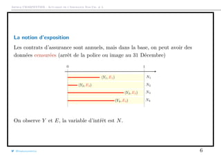
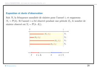
La notion d’exposition
Dans notre base, la fréquence pour les DO est de l’ordre de 6.5%,
1 > Y = freq$nb_DO
2 > E= freq$exposition
3 > sum(Y)/sum(E)
4 [1] 0.06564229
5 > weighted.mean(Y/E,E)
6 [1] 0.06564229
@freakonometrics 7](https://image.slidesharecdn.com/slides-ensae-2016-3-161101132446/85/Slides-ensae-2016-3-7-320.jpg)
![Arthur CHARPENTIER - Actuariat de l’Assurance Non-Vie, # 3
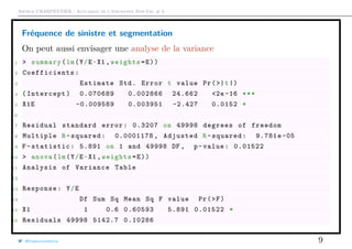
Fréquence de sinistre et segmentation
1 > X1 = freq$carburant
2 > tapply(Y,X1 ,sum)/tapply(E,X1 ,sum)
3 D E
4 0.07068945 0.06110016
5 > library(weights)
6 > wtd.t.test(x=(Y/E)[X1=="D"], y=(Y/E)[X1=="E"],
7 + weight=E[X1=="D"], weighty=E[X1=="E"],samedata=FALSE)
8 $test
9 [1] "Two Sample Weighted T-Test (Welch)"
10
11 $ coefficients
12 t.value df p.value
13 1.768349e+00 2.631555e+04 7.701412e -02
14
15 $ additional
16 Difference Mean.x Mean.y Std. Err
17 0.009589286 0.070689448 0.061100161 0.005422733
@freakonometrics 8](https://image.slidesharecdn.com/slides-ensae-2016-3-161101132446/85/Slides-ensae-2016-3-8-320.jpg)
![Arthur CHARPENTIER - Actuariat de l’Assurance Non-Vie, # 3
Modèle binomial
Le premier modèle auquel on pourrait penser pour modéliser le nombre de
sinistres est le modèle binomial B(n, p). Avec n connu, correspondant à
l’exposition.
Pour être plus précis, on suppose que Yi ∼ B(Ei, pi) où Ei est connu, et où pi est
fonction de variables explicatives (via un lien logistique).
On va exprimer l’exposition en semaine, p est alors la probabilité d’avoir un
sinistre sur une semaine,
1 > freq_b=freq[freq$exposition <=1 ,]
2 > freq_b$sem=round(freq_b$exposition *52)
3 > freq_b=freq_b[freq_b$sem >=1 ,]
Pour faire une régression binomiale (et pas juste Bernoulli)
1 > reg1=glm(nb_DO/sem~1,family=binomial ,weights=sem ,data=freq_b)
ou encore
@freakonometrics 10](https://image.slidesharecdn.com/slides-ensae-2016-3-161101132446/85/Slides-ensae-2016-3-10-320.jpg)
![Arthur CHARPENTIER - Actuariat de l’Assurance Non-Vie, # 3
1 > reg2=glm(cbind(nb_DO , sem -nb_DO) ~ 1, data = freq_b, family =
binomial)
La fréquence annuelle prédite est
1 > predict(reg1 ,type="response")[1]*52
2 1
3 0.06574927
Si on utilise le carburant comme variable de segmentation
1 > reg2 <- glm(cbind(nb_DO , sem -nb_DO) ~ carburant , data = freq_b,
family = binomial)
2 > predict(reg2 ,type="response",newdata=data.frame(carburant=c("D","E"
)))*52
3 1 2
4 0.07097405 0.06104802
Remarque avec une loi binomiale E[N|X] > Var[N|X], sous-dispersion.
@freakonometrics 11](https://image.slidesharecdn.com/slides-ensae-2016-3-161101132446/85/Slides-ensae-2016-3-11-320.jpg)
![Arthur CHARPENTIER - Actuariat de l’Assurance Non-Vie, # 3
La loi de Poisson et période de retour
Supposon qu’un évènement survienne avec une probabilité annuelle p = 1/τ. Soit
T le temps à attendre avant la première survenance,
P[T > n] = 1 −
1
τ
n
∼ e−t/τ
et E[T] = τ (notion de période de retour).
t τ 10 20 50 100 200
10 34.86% 59.87% 81.70% 90.43% 95.11%
20 12.15% 35.84% 66.76% 81.79% 90.46%
50 0.51% 7.69% 36.41% 60.50% 77.83%
100 0.00% 0.59% 13.26% 36.60% 60.57%
200 0.00% 0.00% 1.75% 13.39% 36.69%
@freakonometrics 15](https://image.slidesharecdn.com/slides-ensae-2016-3-161101132446/85/Slides-ensae-2016-3-15-320.jpg)
![Arthur CHARPENTIER - Actuariat de l’Assurance Non-Vie, # 3
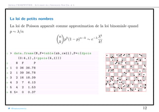
La loi Poisson mélange
En présence de sur-dispersion E(N) < Var(N), on peut penser à une loi Poisson
mélange, i.e. il existe Θ, variable aléatoire positive, avec E(Θ) = 1, telle que
P(N = k|Θ = θ) = e−λθ [λθ]k
k!
, ∀k ∈ N.
0
1
2
3
4
5
6
7
8
9
10
11
12
13
14
15
16
17
18
19
20
21
22
23
24
25
26
27
28
29
30
31
32
33
34
35
36
37
38
39
40
41
42
43
44
45
46
47
48
49
50
0.00
0.02
0.04
0.06
0.08
0.10
Frequence pour la classe (1)
Frequence pour la classe (2)
Frequence du melange
0
1
2
3
4
5
6
7
8
9
10
11
12
13
14
15
16
17
18
19
20
21
22
23
24
25
26
27
28
29
30
31
32
33
34
35
36
37
38
39
40
41
42
43
44
45
46
47
48
49
50
0.00
0.02
0.04
0.06
0.08
Frequence pour la classe (1)
Frequence pour la classe (2)
Frequence du melange
@freakonometrics 17](https://image.slidesharecdn.com/slides-ensae-2016-3-161101132446/85/Slides-ensae-2016-3-17-320.jpg)
![Arthur CHARPENTIER - Actuariat de l’Assurance Non-Vie, # 3
Le processus de Poisson
Pour rappel, (Nt)t≥0 est un processus de Poisson homogène (de paramètre λ) s’il
est à accroissements indépendants, et le nombre de sauts observés pendant la
période [t, t + h] suit une loi P(λ · h).
Ns+1 − Ns ∼ P(λ) est indépendant de Nt+h − Nt ∼ P(λ · h).
@freakonometrics 19](https://image.slidesharecdn.com/slides-ensae-2016-3-161101132446/85/Slides-ensae-2016-3-19-320.jpg)
![Arthur CHARPENTIER - Actuariat de l’Assurance Non-Vie, # 3
Maximum de Vraisemblance
L(λ, Y , E) =
n
i=1
e−λEi
[λEi]Y
i
Yi!
log L(λ, Y , E) = −λ
n
i=1
Ei +
n
i=1
Yi log[λEi] − log
n
i=1
Yi!
qui donne la condition du premier ordre
∂
∂λ
log L(λ, Y , E) = −
n
i=1
Ei +
1
λ
n
i=1
Yi
qui s’annule pour
λ =
n
i=1 Yi
n
i=1 Ei
=
n
i=1
ωi
Yi
Ei
avec ωi =
Ei
n
i=1 Ei
@freakonometrics 21](https://image.slidesharecdn.com/slides-ensae-2016-3-161101132446/85/Slides-ensae-2016-3-21-320.jpg)
![Arthur CHARPENTIER - Actuariat de l’Assurance Non-Vie, # 3
Maximum de Vraisemblance
1 > N = freq$nb_DO
2 > E= freq$exposition
3 > (lambda = sum(N)/sum(E))
4 [1] 0.06564229
5 > dpois (0:3 , lambda)*100
6 [1] 93.646 6.147 0.201 0.004
Remarque: pour Ei on parlera d’exposition ou d’années police.
@freakonometrics 22](https://image.slidesharecdn.com/slides-ensae-2016-3-161101132446/85/Slides-ensae-2016-3-22-320.jpg)
![Arthur CHARPENTIER - Actuariat de l’Assurance Non-Vie, # 3
Fréquence annuelle et une variable tarifaire
1 > X1=freq$carburant
2 > tapply(N,X1 ,sum)
3 D E
4 998 926
5 > tapply(E,X1 ,sum)
6 D E
7 12519.55 13911.58
8 > (lambdas = tapply(N,X1 ,sum)/tapply(E,X1 ,sum))
9 D E
10 0.07971533 0.06656323
11 > cbind(dpois (0:3 , lambdas [1]) ,dpois (0:3 , lambdas [2]))*100
12 [,1] [,2]
13 [1,] 92.337916548 93.560375149
14 [2,] 7.360747674 6.227681197
15 [3,] 0.293382222 0.207267302
16 [4,] 0.007795687 0.004598794
@freakonometrics 23](https://image.slidesharecdn.com/slides-ensae-2016-3-161101132446/85/Slides-ensae-2016-3-23-320.jpg)
![Arthur CHARPENTIER - Actuariat de l’Assurance Non-Vie, # 3
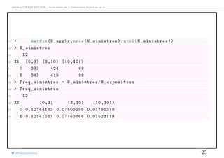
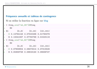
Fréquence annuelle et tableau de contingence
Supposons que l’on prenne en compte ici deux classes de risques.
1 > X1=freq$carburant
2 > X2=cut(freq$agevehicule ,c(0 ,3 ,10 ,101),right=FALSE)
3 > N_polices = table(X1 ,X2)
4 > E_agg=aggregate(E, by = list(X1 = X1 , X2 = X2), sum)
5 > N_exposition=N_polices
6 > N_exposition [1: nrow(N_exposition ) ,1:ncol(N_exposition)]=
7 + matrix(E_agg$x,nrow(N_ exposition),ncol(N_exposition))
8 > N_exposition
9 X2
10 X1 [0 ,3) [3 ,10) [10 ,101)
11 D 3078.938 5653.109 3787.503
12 E 2735.014 5398.950 5777.619
13 >
14 > N_agg=aggregate(N, by = list(X1 = X1 , X2 = X2), sum)
15 > N_sinistres=N_polices
16 > N_sinistres [1: nrow(N_sinistres) ,1:ncol(N_sinistres)]=
@freakonometrics 24](https://image.slidesharecdn.com/slides-ensae-2016-3-161101132446/85/Slides-ensae-2016-3-24-320.jpg)
![Arthur CHARPENTIER - Actuariat de l’Assurance Non-Vie, # 3
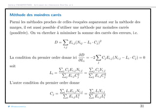
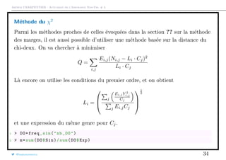
Tableau de contingence et biais minimial
Notons Yi,j le nombre de sinistres observés, Ei,j l’exposition et Ni,j la fréquence
annualisée. La matrice Y = [Yi,j] est ici la fréquence observée. On suppose qu’il
est possible de modéliser Y à l’aide d’un modèle multiplicatif à deux facteurs,
associés à chaque des des variables. On suppose que
Ni,j = Li · Cj, i.e. N = LCT
cf Bailey (1963) et Mildenhall (1999)
L’estimation de L = (Li) et de C = (Cj) se fait généralement de trois manières:
par moindres carrés, par minimisation d’une distance (e.g. du chi-deux) ou par
un principe de balancement (ou méthode des marges).
@freakonometrics 27](https://image.slidesharecdn.com/slides-ensae-2016-3-161101132446/85/Slides-ensae-2016-3-27-320.jpg)

![Arthur CHARPENTIER - Actuariat de l’Assurance Non-Vie, # 3
Méthode des marges, Bailey (1963)
On résoud alors ce petit systeme de maniere itérative (car il n’y a pas de solution
analytique simple).
1 > DO=freq_sin("nb_DO")
2 > m=sum(DO$Sin)/sum(DO$Exp)
3 > L<-matrix(NA ,10, nrow(DO$Exp))
4 > C<-matrix(NA ,10, ncol(DO$Exp))
5 > L[1,] <-rep (1 ,2);colnames(L)=rownames(DO$Sin)
6 > C[1,] <-rep(m,3);colnames(C)=colnames(DO$Sin)
7 >
8 > for(j in 2:10){
9 + L[j ,1] <-sum(DO$Sin [1 ,])/sum(DO$Exp[1,]*C[j-1 ,])
10 + L[j ,2] <-sum(DO$Sin [2 ,])/sum(DO$Exp[2,]*C[j-1 ,])
11 + C[j ,1] <-sum(DO$Sin [ ,1])/sum(DO$Exp[,1]*L[j ,])
12 + C[j ,2] <-sum(DO$Sin [ ,2])/sum(DO$Exp[,2]*L[j ,])
13 + C[j ,3] <-sum(DO$Sin [ ,3])/sum(DO$Exp[,3]*L[j ,])
14 + }
15 > L[10 ,]
@freakonometrics 29](https://image.slidesharecdn.com/slides-ensae-2016-3-161101132446/85/Slides-ensae-2016-3-29-320.jpg)
![Arthur CHARPENTIER - Actuariat de l’Assurance Non-Vie, # 3
16 D E
17 1.007697 1.002415
18 > C[10 ,]
19 [0 ,3) [3 ,10) [10 ,101)
20 0.12593567 0.07588711 0.01623609
21 > PREDICTION =(L[10 ,])%*%t(C[10 ,])
22 > PREDICTION
23 [0 ,3) [3 ,10) [10 ,101)
24 [1,] 0.1269050 0.07647120 0.01636106
25 [2,] 0.1262397 0.07607034 0.01627529
26 > sum(PREDICTION [1,]*DO$Exp [1 ,])
27 [1] 885
28 > sum(DO$Sin [1 ,])
29 [1] 885
@freakonometrics 30](https://image.slidesharecdn.com/slides-ensae-2016-3-161101132446/85/Slides-ensae-2016-3-30-320.jpg)
![Arthur CHARPENTIER - Actuariat de l’Assurance Non-Vie, # 3
On résoud alors ce petit systeme de maniere itérative (car il n’y a pas de solution
analytique simple).
1 > DO=freq_sin("nb_DO")
2 > m=sum(DO$Sin)/sum(DO$Exp)
3 > L<-matrix (1,100, nrow(DO$Exp))
4 > C<-matrix(NA ,100 , ncol(DO$Exp))
5 > L[1,] <-rep (1 ,2);colnames(L)=rownames(DO$Sin)
6 > C[1,] <-rep(m,3);colnames(C)=colnames(DO$Sin)
7 >
8 > for(j in 2:100){
9 + L[j ,1]= sum(DO$Sin [1,]*C[j-1 ,])/sum(DO$Exp[1,]*C[j -1 ,]^2)
10 + L[j ,2]= sum(DO$Sin [2,]*C[j-1 ,])/sum(DO$Exp[2,]*C[j -1 ,]^2)
11 + C[j ,1]= sum(DO$Sin [,1]*L[j ,])/sum(DO$Exp [,1]*L[j ,]^2)
12 + C[j ,2]= sum(DO$Sin [,2]*L[j ,])/sum(DO$Exp [,2]*L[j ,]^2)
13 + C[j ,3]= sum(DO$Sin [,3]*L[j ,])/sum(DO$Exp [,3]*L[j ,]^2)
14 + }
15 >
16 > L[100 ,]
@freakonometrics 32](https://image.slidesharecdn.com/slides-ensae-2016-3-161101132446/85/Slides-ensae-2016-3-32-320.jpg)
![Arthur CHARPENTIER - Actuariat de l’Assurance Non-Vie, # 3
17 D E
18 1.011633 1.012599
19 > C[100 ,]
20 [0 ,3) [3 ,10) [10 ,101)
21 0.12507961 0.07536373 0.01611180
22 > PREDICTION =(L[10 ,])%*%t(C[10 ,])
23 > PREDICTION
24 [0 ,3) [3 ,10) [10 ,101)
25 [1,] 0.1265347 0.07624043 0.01629923
26 [2,] 0.1266554 0.07631321 0.01631479
27 > sum(PREDICTION [1,]*DO$Exp [1 ,])
28 [1] 882.3211
29 > sum(DO$Sin [1 ,])
30 [1] 885
@freakonometrics 33](https://image.slidesharecdn.com/slides-ensae-2016-3-161101132446/85/Slides-ensae-2016-3-33-320.jpg)
![Arthur CHARPENTIER - Actuariat de l’Assurance Non-Vie, # 3
3 > L<-matrix (1,100, nrow(DO$Exp))
4 > C<-matrix(NA ,100 , ncol(DO$Exp))
5 > L[1,] <-rep (1 ,2);colnames(L)=rownames(DO$Sin)
6 > C[1,] <-rep(m,3);colnames(C)=colnames(DO$Sin)
7 >
8 > for(j in 2:100){
9 + L[j ,1]= sqrt(sum(DO$Exp[1,]*DO$Freq [1 ,]^2/C[j-1 ,])/sum(DO$Exp[1,]*C
[j-1 ,]))
10 + L[j ,2]= sqrt(sum(DO$Exp[2,]*DO$Freq [2 ,]^2/C[j-1 ,])/sum(DO$Exp[2,]*C
[j-1 ,]))
11 + C[j ,1]= sqrt(sum(DO$Exp[,1]*DO$Freq [ ,1]^2/L[j ,])/sum(DO$Exp [,1]*L[j
,]))
12 + C[j ,2]= sqrt(sum(DO$Exp[,2]*DO$Freq [ ,2]^2/L[j ,])/sum(DO$Exp [,2]*L[j
,]))
13 + C[j ,3]= sqrt(sum(DO$Exp[,3]*DO$Freq [ ,3]^2/L[j ,])/sum(DO$Exp [,3]*L[j
,]))
14 + }
15 >
@freakonometrics 35](https://image.slidesharecdn.com/slides-ensae-2016-3-161101132446/85/Slides-ensae-2016-3-35-320.jpg)
![Arthur CHARPENTIER - Actuariat de l’Assurance Non-Vie, # 3
16 > L[100 ,]
17 D E
18 1.19012 1.18367
19 > C[100 ,]
20 [0 ,3) [3 ,10) [10 ,101)
21 0.10664299 0.06427321 0.01379165
22 > PREDICTION =(L[10 ,])%*%t(C[10 ,])
23 > PREDICTION
24 [0 ,3) [3 ,10) [10 ,101)
25 [1,] 0.1269180 0.07649285 0.01641373
26 [2,] 0.1262301 0.07607824 0.01632476
27 > sum(PREDICTION [1,]*DO$Exp [1 ,])
28 [1] 885.362
29 > sum(DO$Sin [1 ,])
30 [1] 885
(on est très proche ici de la méthode des marges, de Bailey).
@freakonometrics 36](https://image.slidesharecdn.com/slides-ensae-2016-3-161101132446/85/Slides-ensae-2016-3-36-320.jpg)
![Arthur CHARPENTIER - Actuariat de l’Assurance Non-Vie, # 3
Approche(s) économétrique(s) du biais minimal
Ici, on considère y = [Ni,j] et y = [LiCj] = [e i+cj
].
Rappel Dans un modèle linéaire - i.e. E[Y ] = Xβ - avec homoscédasticité, les
équations normales sont
XT
[y − Xβ] = 0
et dans un modèle avec hétéroscédasticité, si Var[ε] = σ2
Ω,
XT
Ω−1
[y − Xβ] = 0
Dans un modèle multiplicatif - E[Y ] = eXβ
avec homoscédasticité, les équations
normales sont
XT
eXβ
[y − eXβ
] = 0
et dans un modèle avec hétéroscédasticité, si Var[ε] = σ2
Ω,
XT
Ω−1
eXβ
[y − eXβ
] = 0
@freakonometrics 37](https://image.slidesharecdn.com/slides-ensae-2016-3-161101132446/85/Slides-ensae-2016-3-37-320.jpg)
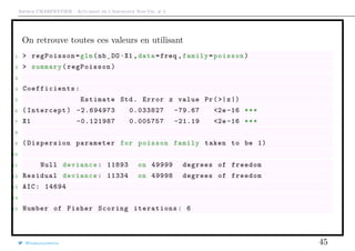
![Arthur CHARPENTIER - Actuariat de l’Assurance Non-Vie, # 3
Approche(s) économétrique(s) du biais minimal
Résoudre XT
[y − eXβ
] = 0 revient à considérer un modèle multiplicatif,
hétéroscedastique, avec Ω ∝ eXβ
, i.e. Var(Y ) ∝ E[Y ] (cf loi de Poisson).
1 > df_agg=data.frame(N=as.numeric(DO$Sin),E=as.numeric(DO$Exp), X1=rep
(levels(X1),ncol(DO$Sin)),X2=rep(levels(X2),each=nrow(DO$Sin)))
2 > regpoislog_agg <- glm(N~X1+X2 ,offset=log(E),data=df_agg , family=
poisson(link="log"))
3 > ndf_agg=df_agg
4 > ndf_agg$E=1
5 > matrix(predict(regpoislog_agg ,type="response",newdata=ndf_agg),nrow
(PREDICTION),ncol(PREDICTION ))
6 [,1] [,2] [,3]
7 [1,] 0.1269050 0.07647120 0.01636106
8 [2,] 0.1262397 0.07607034 0.01627529
@freakonometrics 38](https://image.slidesharecdn.com/slides-ensae-2016-3-161101132446/85/Slides-ensae-2016-3-38-320.jpg)
![Arthur CHARPENTIER - Actuariat de l’Assurance Non-Vie, # 3
Approche(s) économétrique(s) du biais minimal
ou au niveau individuel
1 > df=data.frame(N=freq[,"nb_DO"],E,X1 ,X2)
2 > regpoislog <- glm(N~X1+X2 ,offset=log(E),data=df , family=poisson(
link="log"))
3 > rownames(PREDICTION)=c("D","E")
4 > newd <- data.frame(X1=factor(rep(rownames(PREDICTION),ncol(
PREDICTION))), E=rep (1 ,6), X1=factor(rep(rownames(PREDICTION),ncol
(PREDICTION))), X2=factor(rep(colnames( PREDICTION),each=nrow(
PREDICTION))))
5 > matrix(predict(regpoislog ,newdata=newd ,
6 + type="response"),nrow(PREDICTION),ncol(PREDICTION))
7 [,1] [,2] [,3]
8 [1,] 0.1269050 0.07647120 0.01636106
9 [2,] 0.1262397 0.07607034 0.01627529
@freakonometrics 39](https://image.slidesharecdn.com/slides-ensae-2016-3-161101132446/85/Slides-ensae-2016-3-39-320.jpg)
![Arthur CHARPENTIER - Actuariat de l’Assurance Non-Vie, # 3
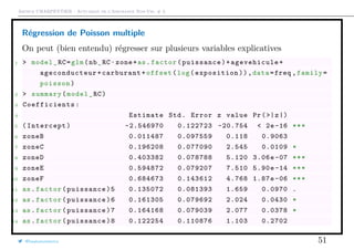
Approche(s) économétrique(s) du biais minimal
On peut aussi envisager un modèle homosc´dastique
1 > df_agg=data.frame(N=as.numeric(DO$Sin),E=as.numeric(DO$Exp), X1=rep
(levels(X1),ncol(DO$Sin)),X2=rep(levels(X2),each=nrow(DO$Sin)))
2 > reggauss_agg <- glm(N~X1+X2 ,offset=log(E),family=gaussian(link="log
"),data=df_agg)
3 > ndf_agg=df_agg
4 > ndf_agg$E=1
5 > matrix(predict(reggauss_agg ,type="response",newdata=ndf_agg),nrow(
PREDICTION),ncol(PREDICTION))
6 [,1] [,2] [,3]
7 [1,] 0.1261529 0.07592604 0.01594451
8 [2,] 0.1272804 0.07660463 0.01608701
@freakonometrics 40](https://image.slidesharecdn.com/slides-ensae-2016-3-161101132446/85/Slides-ensae-2016-3-40-320.jpg)
![Arthur CHARPENTIER - Actuariat de l’Assurance Non-Vie, # 3
La régression de Poisson
L’idée est la même que pour la régression logistique: on cherche un modèle
linéaire pour la moyenne. En l’occurence,
Yi ∼ P(λi) avec λi = exp[Xiβ].
Dans ce modèle, E(Yi|Xi) = Var(Yi|Xi) = λi = exp[Xiβ].
Remarque: on posera parfois θi = ηi = Xiβ
La log-vraisemblance est ici
log L(β; Y ) =
n
i=1
[Yi log(λi) − λi − log(Yi!)]
ou encore
log L(β; Y ) =
n
i=1
Yi · [Xiβ] − exp[Xiβ] − log(Yi!)
@freakonometrics 41](https://image.slidesharecdn.com/slides-ensae-2016-3-161101132446/85/Slides-ensae-2016-3-41-320.jpg)
![Arthur CHARPENTIER - Actuariat de l’Assurance Non-Vie, # 3
Le gradient est ici
log L(β; Y ) =
∂ log L(β; Y )
∂β
=
n
i=1
(Yi − exp[Xiβ])Xi
alors que la matrice Hessienne s’écrit
H(β) =
∂2
log L(β; Y )
∂β∂β
= −
n
i=1
(Yi − exp[Xiβ])XiXi
La recherche du maximum de log L(β; Y ) est obtenu (numériquement) par
l’algorithme de Newton-Raphson,
1. partir d’une valeur initiale β0
2. poser βk = βk−1 − H(βk−1)−1
log L(βk−1)
où log L(β) est le gradient, et H(β) la matrice Hessienne (on parle parfois de
Score de Fisher).
@freakonometrics 42](https://image.slidesharecdn.com/slides-ensae-2016-3-161101132446/85/Slides-ensae-2016-3-42-320.jpg)
![Arthur CHARPENTIER - Actuariat de l’Assurance Non-Vie, # 3
La régression de Poisson
Par exemple, si on régresse sur l’âge du véhicule
1 > Y <- freq$nb_DO
2 > X1 <- freq$agevehicule
3 > X <- cbind(rep(1, length(X1)),X1)
on part d’une valeur initiale (e.g. une estimation classique de modèle linéaire)
1 > beta=lm(Y~0+X)$ coefficients
On fait ensuite une boucle (avec 50,000 lignes, l’algorithme du cours #2. ne
fonctionne pas)
1 > for(s in 1:20){
2 + gradient=t(X)%*%(Y-exp(X%*%beta))
3 + hessienne=matrix (0,ncol(X),ncol(X))
4 + for(i in 1: nrow(X)){
5 + hessienne=hessienne + as.numeric(exp(X[i,]%*%beta))* (X[i,]%*%t(X[i
,]))}
@freakonometrics 43](https://image.slidesharecdn.com/slides-ensae-2016-3-161101132446/85/Slides-ensae-2016-3-43-320.jpg)
![Arthur CHARPENTIER - Actuariat de l’Assurance Non-Vie, # 3
6 + beta=beta+solve(hessienne)%*%gradient
7 + }
On peut montrer que β
P
→ β et
√
n(β − β)
L
→ N(0, I(β)−1
).
Numériquement, la encore, on peut approcher I(β)−1
qui est la variance
(asymptotique) de notre estimateur. Or I(β) = H(β), donc les écart-types de β
donnés à droite
1 > cbind(beta ,sqrt(diag(solve(hessienne))))
2 [,1] [,2]
3 -2.6949729 0.03382691
4 X1 -0.1219873 0.00575687
@freakonometrics 44](https://image.slidesharecdn.com/slides-ensae-2016-3-161101132446/85/Slides-ensae-2016-3-44-320.jpg)
![Arthur CHARPENTIER - Actuariat de l’Assurance Non-Vie, # 3
Loi de Poisson vs. Conditions du Premier Ordre
D’un point de vue computationnel, l’ordinateur cherche à résoudre
XT
[y − exp(Xβ)] = 0, i.e.
n
i=1
XT
i [y − exp(XT
i β)] = 0
À aucun moment, on a besoin d’avoir yi ∈ N. En fait, on peut faire une
‘régression de Poisson’ pour des variables non-entières.
1 > reg=glm(nb_RC~1,data=freq ,family=poisson)
2 > predict(reg ,type="response")[1]
3 1
4 0.03848
5 > reg=glm(nb_RC/10~1,data=freq ,family=poisson)
6 There were 50 or more warnings (use warnings () to see the first 50)
7 > predict(reg ,type="response")[1]
8 1
9 0.003848
@freakonometrics 46](https://image.slidesharecdn.com/slides-ensae-2016-3-161101132446/85/Slides-ensae-2016-3-46-320.jpg)
![Arthur CHARPENTIER - Actuariat de l’Assurance Non-Vie, # 3
Propriété de la Régression de Poisson
Les conditions du premier ordre XT
[y − exp(Xβ)] = 0 peuvent s’écrire
XT
y = XT
exp(Xβ) ou encore XT
y.
S’il y a une constante, la première colonne implique
1T
y = 1T
y i.e.
n
i=1
yi =
n
i=1
yi
Si X est une variable factorielle de modalités a1, · · · , aJ ,
1T
aj
y = 1T
aj
y i.e.
i;xi=aj
yi =
i;xi=aj
yi
@freakonometrics 47](https://image.slidesharecdn.com/slides-ensae-2016-3-161101132446/85/Slides-ensae-2016-3-47-320.jpg)
![Arthur CHARPENTIER - Actuariat de l’Assurance Non-Vie, # 3
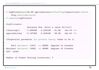
Prise en compte de l’exposition (offset)
Oups, on a oublié de prendre l’exposition dans notre modèle. On a ajusté un
modèle de la forme
Yi ∼ P(λi) avec λi = exp[β0 + β1X1,i]
mais on voudrait
Yi ∼ P(λi · Ei) avec λi = exp[β0 + β1X1,i]
ou encore
Yi ∼ P(˜λi) avec ˜λi = Ei · exp[β0 + β1X1,i] = exp[β0 + β1X1,i + log(Ei)]
Aussi, l’exposition intervient comme une variable de la régression, mais en
prenant le logarithme de l’exposition, et en forçant le paramètre à être unitaire,
i.e.
Yi ∼ P(˜λi) avec ˜λi = Ei · exp[β0 + β1X1,i] = exp[β0 + β1X1,i + 1 log(Ei)]
@freakonometrics 48](https://image.slidesharecdn.com/slides-ensae-2016-3-161101132446/85/Slides-ensae-2016-3-48-320.jpg)
![Arthur CHARPENTIER - Actuariat de l’Assurance Non-Vie, # 3
1 > Y <- freq$nb_DO
2 > X1 <- freq$agevehicule
3 > E <- freq$exposition
4 > X=cbind(rep(1, length(X1)),X1)
5 > beta=lm(Y~0+X)$ coefficients
6 > for(s in 1:20){
7 + gradient=t(X)%*%(Y-exp(X%*%beta+log(E)))
8 + hessienne=matrix (0,ncol(X),ncol(X))
9 + for(i in 1: nrow(X)){
10 + hessienne=hessienne + as.numeric(exp(X[i,]%*%beta+log(E[i])))*(
X[i,]%*%t(X[i,]))}
11 + beta=beta+solve(hessienne)%*%gradient
12 + }
13 >
14 > cbind(beta ,sqrt(diag(solve(hessienne))))
15 [,1] [,2]
16 -1.8256863 0.035138680
17 X1 -0.1578027 0.006198479
@freakonometrics 49](https://image.slidesharecdn.com/slides-ensae-2016-3-161101132446/85/Slides-ensae-2016-3-49-320.jpg)
![Arthur CHARPENTIER - Actuariat de l’Assurance Non-Vie, # 3
Effets marginaux, et élasticité
Les effets marginaux de la variable k pour l’individu i sont donnés par
∂E(Yi|Xi)
∂Xi,k
=
∂ exp[XT
i β]
∂Xk
= exp[XT
i β] · βk
estimés pas exp[Xiβ] · βk
Par exemple, pour avoir l’effet marginal de la variable ageconducteur,
1 > coef(model_RC)[19]
2 ageconducteur
3 -0.008844096
4 > effet19=predict(model_DO ,type="response")*coef(model_RC)[19]
5 > effet19 [1:4]
6 1 2 3 4
7 -1.188996e -03 -1.062340e-03 -7.076257e -05 -2.367111e-04
@freakonometrics 53](https://image.slidesharecdn.com/slides-ensae-2016-3-161101132446/85/Slides-ensae-2016-3-53-320.jpg)
![Arthur CHARPENTIER - Actuariat de l’Assurance Non-Vie, # 3
Effets marginaux, et élasticité
On peut aussi calculer les effets marginaux moyens de la variable k, Y · βk
1 > mean(predict(model_RC ,type="response"))*coef(model_RC)[19]
2 ageconducteur
3 -0.0003403208
Autrement dit, en vieillissant d’un an, il y aura (en moyenne) 0.0003 accident de
moins, par an, par assuré.
Ici, on utilise des changements en unité (∂Xi,k), mais il est possible détudier
l’impact de changement en proportion. Au lieu de varier d’une utilité, on va
considérer un changement de 1%.
@freakonometrics 54](https://image.slidesharecdn.com/slides-ensae-2016-3-161101132446/85/Slides-ensae-2016-3-54-320.jpg)
![Arthur CHARPENTIER - Actuariat de l’Assurance Non-Vie, # 3
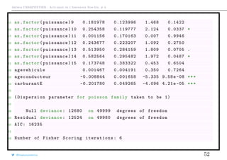
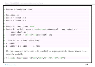
Interprétation, suite
Dans la sortie, nous avons obtenu
1 Coefficients :
2 Estimate Std. Error z value Pr(>|z|)
...
1 carburantE -0.201780 0.049265 -4.096 4.21e -05 ***
i.e.
23 > coefficients (model_RC)["carburantE "]
24 carburantE
25 -0.2017798
Autrement dit, à caractéristiques identiques, un assuré conduisant un véhicule
essence a une fréquence de sinistres presque 20% plus faible qu’un assuré
conduisant un véhicule diesel,
1 > exp( coefficients (model_RC)["carburantE "])
@freakonometrics 55](https://image.slidesharecdn.com/slides-ensae-2016-3-161101132446/85/Slides-ensae-2016-3-55-320.jpg)


![Arthur CHARPENTIER - Actuariat de l’Assurance Non-Vie, # 3
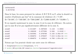
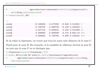
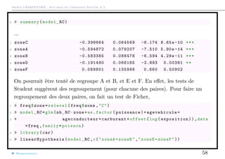
Variable Explicative Spatiale
Les régions utilisées sur la base sont reliées à la classification INSEE, data.gouv.fr
1 > loc="http://osm13. openstreetmap .fr/~cquest/openfla/export/regions
-20140306 -5m-shp.zip"
2 > download.file(loc ,"region.zip")
3 > unzip("region.zip",exdir="regions")
4 > require(maptools)
5 > regions= readShapePoly ("./regions/regions -20140306 -5m.shp")
6 > LISTE= regions@data $nom[
7 c(1 ,2 ,3 ,4 ,5 ,6 ,7 ,8 ,9 ,10 ,13 ,14 ,15 ,17 ,18 ,21 ,22 ,23 ,24 ,25 ,26 ,27)]
8 > corresp_insee=
9 c(42 ,72 ,83 ,25 ,26 ,53 ,24 ,21 ,94 ,43 ,23 ,11 ,91 ,74 ,41 ,73 ,31 ,52 ,22 ,54 ,93 ,82)
@freakonometrics 64](https://image.slidesharecdn.com/slides-ensae-2016-3-161101132446/85/Slides-ensae-2016-3-64-320.jpg)
![Arthur CHARPENTIER - Actuariat de l’Assurance Non-Vie, # 3
Variable Explicative Spatiale
1 > N = freq$nb_RC
2 > E= freq$exposition
3 > X1=freq$region
4 > T=tapply(N,X1 ,sum)/tapply(E,X1 ,sum)
5 > T=T[as.character(corresp_insee)]
6 > library( RColorBrewer )
7 > CLpalette= colorRampPalette (rev(brewer
.pal(n = 9, name = "RdYlBu")))(100)
8 > lst=which( regions@data $nom%in%LISTE)
9 > plot(regions[lst ,],col=CLpalette[
round(T/.15*100) ])
qqqqqqqqqqqqqqqqqqqqqqqqqqqqqqqqqqqqqqqqqqqqqqqqqqqqqqqqqqqqqqqqqqqqqqqqqqqqqqqqqqqqqqqqqqqqqqqqqqqq
0.00 0.05 0.10 0.15
@freakonometrics 65](https://image.slidesharecdn.com/slides-ensae-2016-3-161101132446/85/Slides-ensae-2016-3-65-320.jpg)
![Arthur CHARPENTIER - Actuariat de l’Assurance Non-Vie, # 3
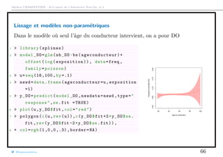
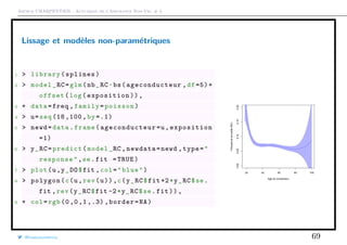
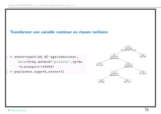
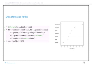
Transformer une variable continue en classes tarifaires
On peut envisager un découpage exogène, e.g. par intervalles de taille ´gale
1 > library(classInt)
2 > CI= classIntervals (freq$ageconducteur , 6,
style = "equal",intervalClosure ="left")
3 > LV=CI$brks
4 > LV [6]= LV [6]+1
5 > graph_freq(" ageconducteur ",levels=LV) [18,31.7] (31.7,45.3] (45.3,59] (59,72.7] (72.7,87.3] (87.3,100]
05000100001500020000
0.000.050.10
Exposure
AnnualizedFrequency
@freakonometrics 71](https://image.slidesharecdn.com/slides-ensae-2016-3-161101132446/85/Slides-ensae-2016-3-71-320.jpg)
![Arthur CHARPENTIER - Actuariat de l’Assurance Non-Vie, # 3
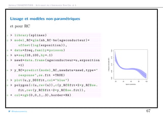
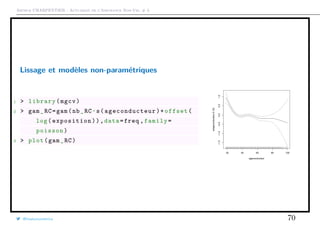
Transformer une variable continue en classes tarifaires
ou par intervalles basés sur les quantiles
1 > library(classInt)
2 > CI= classIntervals (freq$ageconducteur , 6,
style = "quantile",intervalClosure ="left
")
3 > LV=CI$brks
4 > LV [6]= LV [6]+1
5 > graph_freq(" ageconducteur ",levels=LV)
[18,31] (31,38] (38,44] (44,51] (51,60] (60,100]
020004000600080001000012000
0.050.10
Exposure
AnnualizedFrequency
@freakonometrics 72](https://image.slidesharecdn.com/slides-ensae-2016-3-161101132446/85/Slides-ensae-2016-3-72-320.jpg)
![Arthur CHARPENTIER - Actuariat de l’Assurance Non-Vie, # 3
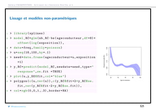
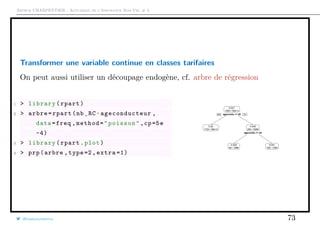
Transformer une variable continue en classes tarifaires
1 > lb=labels(arbre)
2 > cut_ages = substr(lb ,nchar(lb) -3,
nchar(lb))
3 > cut_ages=as.numeric(cut_ages)
4 > LV=c(18, sort(unique(cut_ages[!is.na
(cut_ages)])) ,101)
5 > graph_freq(" ageconducteur ",levels=
LV) [18,23.5] (23.5,26.5] (26.5,51.5] (51.5,53.5] (53.5,101]
05000150002500035000
0.000.050.100.150.20
Exposure
AnnualizedFrequency
@freakonometrics 75](https://image.slidesharecdn.com/slides-ensae-2016-3-161101132446/85/Slides-ensae-2016-3-75-320.jpg)
![Arthur CHARPENTIER - Actuariat de l’Assurance Non-Vie, # 3
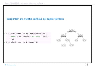
Transformer une variable continue en classes tarifaires
1 > lb=labels(arbre)
2 > cut_ages = substr(lb ,nchar(lb) -3,
nchar(lb))
3 > cut_ages=as.numeric(cut_ages)
4 > LV=c(18, sort(unique(cut_ages[!is.na
(cut_ages)])) ,101)
5 > graph_freq(" ageconducteur ",levels=
LV) [18,26.5] (26.5,37.5] (37.5,41.5] (41.5,53.5] (53.5,101]
05000100001500020000
0.050.100.15
Exposure
AnnualizedFrequency
@freakonometrics 77](https://image.slidesharecdn.com/slides-ensae-2016-3-161101132446/85/Slides-ensae-2016-3-77-320.jpg)
![Arthur CHARPENTIER - Actuariat de l’Assurance Non-Vie, # 3
Arbre pour une loi de Poisson ?
On utilise ici une fonction d’impureté I(·) basé sur la déviance de la loi de
Poisson. Pour un noeud N,
I(N) =
i∈{N}
Yi log
Yi
λN Ei
− [Yi − λN Ei] avec λN =
i∈{N} Yi
i∈{N} Ei
La méthode est ensuite la même que pour un arbre de classification.
la log-vraisemblance pour une loi de Poisson est
log L(λ) =
n
i=1
yi log λi − λi − log(yi!)
et la déviance est alors la différence
log L(y) − log L(λ) =
n
i=1
yi log
yi
λi
− [yi − λi]
@freakonometrics 78](https://image.slidesharecdn.com/slides-ensae-2016-3-161101132446/85/Slides-ensae-2016-3-78-320.jpg)

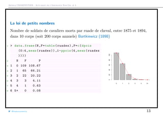
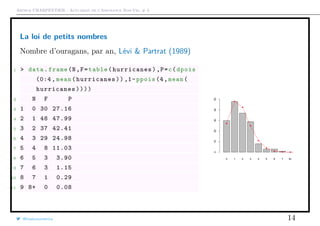
Le document présente des méthodes de modélisation économétrique pour l'assurance non-vie, en se concentrant sur des variables de comptage et notamment la régression de Poisson. Il inclut des analyses de données de sinistres et d'exposition, ainsi que des modèles binomiaux pour estimer la fréquence des sinistres. Diverses approches, dont la loi de Poisson et la loi binomiale négative, sont discutées pour décrire les phénomènes observés dans les contrats d'assurance.


