Télécharger en tant que PDF, PPTX
![Arthur CHARPENTIER - ACT2040 - Actuariat IARD - Hiver 2013
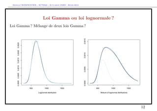
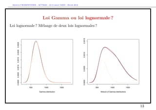
Modélisation de variables positives
Références : Frees (2010), chapitre 13, de Jong & Heller (2008), chapitre 8, et
Denuit & Charpentier (2005), chapitre 11.
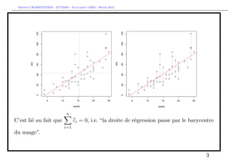
n n
Préambule : avec le modèle linéaire, nous avions Yi = Yi
i=1 i=1
> reg=lm(dist~speed,data=cars)
> sum(cars$dist)
[1] 2149
> sum(predict(reg))
[1] 2149
2](https://image.slidesharecdn.com/slides-2040-6-130215130733-phpapp01/85/Slides-2040-6-2-320.jpg)
![Arthur CHARPENTIER - ACT2040 - Actuariat IARD - Hiver 2013
Cette propriété était conservée avec la régression log-Poisson, nous avions que
n n
Yi = µi Ei , où µi Ei est la prédiction faite avec l’exposition, au sens où
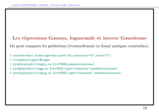
i=1 i=1
> sum(sinistres$nbre)
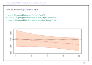
[1] 1924
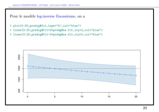
> reg=glm(nbre~1+offset(log(exposition)),data=sinistres,
+ family=poisson(link="log"))
> sum(predict(reg,type="response"))
[1] 1924
> sum(predict(reg,newdata=data.frame(exposition=1),
+ type="response")*sinistres$exposition)
[1] 1924
et ce, quel que soit le modèle utilisé !
> reg=glm(nbre~offset(log(exposition))+ageconducteur+
+ zone+carburant,data=sinistres,family=poisson(link="log"))
> sum(predict(reg,type="response"))
[1] 1924
4](https://image.slidesharecdn.com/slides-2040-6-130215130733-phpapp01/85/Slides-2040-6-4-320.jpg)
![Arthur CHARPENTIER - ACT2040 - Actuariat IARD - Hiver 2013
... mais c’est tout. En particulier, cette propriété n’est pas vérifiée si on change de
fonction lien,
> reg=glm(nbre~1+log(exposition),data=sinistres,
> sum(predict(reg,type="response"))
[1] 1977.704
ou de loi (e.g. binomiale négative),
> reg=glm.nb(nbre~1+log(exposition),data=sinistres)
> sum(predict(reg,type="response"))
[1] 1925.053
n n
Conclusion : de manière générale Yi = Yi
i=1 i=1
5](https://image.slidesharecdn.com/slides-2040-6-130215130733-phpapp01/85/Slides-2040-6-5-320.jpg)
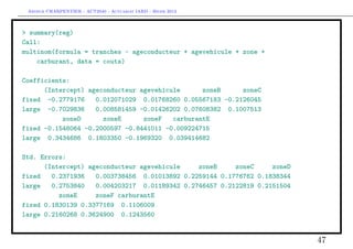
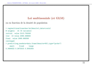
![Arthur CHARPENTIER - ACT2040 - Actuariat IARD - Hiver 2013
La base des coûts individuels
> sinistre=read.table("http://freakonometrics.free.fr/sinistreACT2040.txt",
+ header=TRUE,sep=";")
> sinistres=sinistre[sinistre$garantie=="1RC",]
> sinistres=sinistres[sinistres$cout>0,]
> contrat=read.table("http://freakonometrics.free.fr/contractACT2040.txt",
+ header=TRUE,sep=";")
> couts=merge(sinistres,contrat)
> tail(couts,4)
nocontrat no garantie cout exposition zone puissance agevehicule
1921 6108364 13229 1RC 1320.0 0.74 B 9 1
1922 6109171 11567 1RC 1320.0 0.74 B 13 1
1923 6111208 14161 1RC 970.2 0.49 E 10 5
1924 6111650 14476 1RC 1940.4 0.48 E 4 0
ageconducteur bonus marque carburant densite region
1921 32 100 12 E 83 0
1922 56 50 12 E 93 13
1923 30 90 12 E 53 2
1924 69 50 12 E 93 13
6](https://image.slidesharecdn.com/slides-2040-6-130215130733-phpapp01/85/Slides-2040-6-6-320.jpg)
![Arthur CHARPENTIER - ACT2040 - Actuariat IARD - Hiver 2013
La loi Gamma
La densité de Y est ici
φ−1
1 y y
f (y) = exp − , ∀y ∈ R+
yΓ(φ−1 ) µφ µφ
qui est dans la famille exponentielle, puisque
y/µ − (− log µ) 1 − φ log φ
f (y) = + log y − − log Γ φ−1 , ∀y ∈ R+
−φ φ φ
On en déduit en particulier le lien canonique, θ = µ−1 (fonction de lien inverse).
De plus, b(θ) = − log(µ), de telle sorte que b (θ) = µ et b (θ) = −µ2 . La fonction
variance est alors ici V (µ) = µ2 .
Enfin, la déviance est ici
n
yi − µi yi
D = 2φ[log L(y, y) − log L(µ, y)] = 2φ − log .
i=1
µi µi
7](https://image.slidesharecdn.com/slides-2040-6-130215130733-phpapp01/85/Slides-2040-6-7-320.jpg)
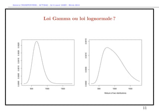
![Arthur CHARPENTIER - ACT2040 - Actuariat IARD - Hiver 2013
La loi lognormale
La densité de Y est ici
1 −
(ln y−µ)2
f (y) = y √ e 2σ 2 , ∀y ∈ R+
y 2πσ 2
Si Y suit une loi lognormale de paramètres µ et σ 2 , alors Y = exp[Y ] où
Y ∼ N (µ, σ 2 ). De plus,
E(Y ) = E(exp[Y ]) = exp [E(Y )] = exp(µ).
µ+σ 2 /2 σ2 2µ+σ 2
Rappelons que E(Y ) = e , et Var(Y ) = (e − 1)e .
> plot(cars)
> regln=lm(log(dist)~speed,data=cars)
> nouveau=data.frame(speed=1:30)
> preddist=exp(predict(regln,newdata=nouveau))
8](https://image.slidesharecdn.com/slides-2040-6-130215130733-phpapp01/85/Slides-2040-6-8-320.jpg)
![Arthur CHARPENTIER - ACT2040 - Actuariat IARD - Hiver 2013
> lines(1:30,preddist,col="red")
> (s=summary(regln)$sigma)
[1] 0.4463305
> lines(1:30,preddist*exp(.5*s^2),col="blue")
9](https://image.slidesharecdn.com/slides-2040-6-130215130733-phpapp01/85/Slides-2040-6-9-320.jpg)
![Arthur CHARPENTIER - ACT2040 - Actuariat IARD - Hiver 2013
n n n
σ2
Remarque on n’a pas, pour autant, Yi = Yi = exp Yi +
i=1 i=1 i=1
2
> sum(cars$dist)
[1] 2149
> sum(exp(predict(regln)))
[1] 2078.34
> sum(exp(predict(regln))*exp(.5*s^2))
[1] 2296.015
même si on ne régresse sur aucune variable explicative...
> regln=lm(log(dist)~1,data=cars)
> (s=summary(regln)$sigma)
[1] 0.7764719
> sum(exp(predict(regln))*exp(.5*s^2))
[1] 2320.144
10](https://image.slidesharecdn.com/slides-2040-6-130215130733-phpapp01/85/Slides-2040-6-10-320.jpg)
![Arthur CHARPENTIER - ACT2040 - Actuariat IARD - Hiver 2013
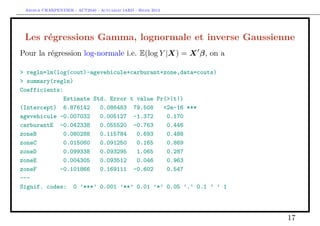
Les régressions Gamma, lognormale et inverse Gaussienne
Pour la régression Gamma (et un lien log i.e. E(Y |X) = exp[X β]), on a
> regg=glm(cout~agevehicule+carburant+zone,data=couts,
+ family=Gamma(link="log"))
> summary(regg)
Coefficients:
Estimate Std. Error t value Pr(>|t|)
(Intercept) 8.17615 0.22937 35.646 <2e-16 ***
agevehicule -0.01715 0.01360 -1.261 0.2073
carburantE -0.20756 0.14725 -1.410 0.1588
zoneB -0.60169 0.30708 -1.959 0.0502 .
zoneC -0.60072 0.24201 -2.482 0.0131 *
zoneD -0.45611 0.24744 -1.843 0.0654 .
zoneE -0.43725 0.24801 -1.763 0.0781 .
zoneF 0.24778 0.44852 0.552 0.5807
---
Signif. codes: 0 ’***’ 0.001 ’**’ 0.01 ’*’ 0.05 ’.’ 0.1 ’ ’ 1
(Dispersion parameter for Gamma family taken to be 9.91334)
15](https://image.slidesharecdn.com/slides-2040-6-130215130733-phpapp01/85/Slides-2040-6-15-320.jpg)
![Arthur CHARPENTIER - ACT2040 - Actuariat IARD - Hiver 2013
Les régressions Gamma, lognormale et inverse Gaussienne
Pour la régression inverse-Gaussienne, (et un lien log i.e. E(Y |X) = exp[X β]),
> regig=glm(cout~agevehicule+carburant+zone,data=couts,
+ family=inverse.gaussian(link="log"),start=coefficients(regg))
> summary(regig)
Coefficients:
Estimate Std. Error t value Pr(>|t|)
(Intercept) 8.07065 0.23606 34.188 <2e-16 ***
agevehicule -0.01509 0.01118 -1.349 0.1774
carburantE -0.18037 0.13065 -1.381 0.1676
zoneB -0.50202 0.28836 -1.741 0.0819 .
zoneC -0.50913 0.24098 -2.113 0.0348 *
zoneD -0.38080 0.24806 -1.535 0.1249
zoneE -0.36541 0.24975 -1.463 0.1436
zoneF 0.42854 0.56537 0.758 0.4486
---
Signif. codes: 0 ’***’ 0.001 ’**’ 0.01 ’*’ 0.05 ’.’ 0.1 ’ ’ 1
(Dispersion parameter for inverse.gaussian family taken to be 0.004331898)
16](https://image.slidesharecdn.com/slides-2040-6-130215130733-phpapp01/85/Slides-2040-6-16-320.jpg)
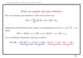
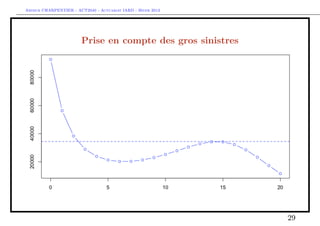
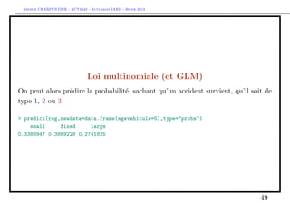
![Arthur CHARPENTIER - ACT2040 - Actuariat IARD - Hiver 2013
Prise en compte des gros sinistres
Pour le terme B, il s’agit d’une régression standard d’une variable de Bernoulli,
> s = 10000
> couts$normal=(couts$cout<=s)
> mean(couts$normal)
[1] 0.9818087
> library(splines)
> age=seq(0,20)
> regC=glm(normal~bs(agevehicule),data=couts,family=binomial)
> ypC=predict(regC,newdata=data.frame(agevehicule=age),type="response")
> plot(age,ypC,type="b",col="red")
> regC2=glm(normal~1,data=couts,family=binomial)
> ypC2=predict(regC2,newdata=data.frame(agevehicule=age),type="response")
> lines(age,ypC2,type="l",col="red",lty=2)
24](https://image.slidesharecdn.com/slides-2040-6-130215130733-phpapp01/85/Slides-2040-6-24-320.jpg)
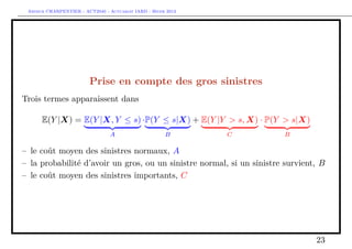
![Arthur CHARPENTIER - ACT2040 - Actuariat IARD - Hiver 2013
Prise en compte des gros sinistres
Pour le terme A, il s’agit d’une régression standard sur la base restreinte,
> indice = which(couts$cout<=s)
> mean(couts$cout[indice])
[1] 1335.878
> library(splines)
> regA=glm(cout~bs(agevehicule),data=couts,
+ subset=indice,family=Gamma(link="log"))
> ypA=predict(regA,newdata=data.frame(agevehicule=age),type="response")
> plot(age,ypA,type="b",col="red")
> ypA2=mean(couts$cout[indice])
> abline(h=ypA2,lty=2,col="red")
26](https://image.slidesharecdn.com/slides-2040-6-130215130733-phpapp01/85/Slides-2040-6-26-320.jpg)
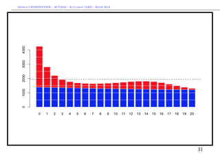
![Arthur CHARPENTIER - ACT2040 - Actuariat IARD - Hiver 2013
Prise en compte des gros sinistres
Pour le terme C, il s’agit d’une régression standard sur la base restreinte,
> indice = which(couts$cout>s)
> mean(couts$cout[indice])
[1] 34471.59
> regB=glm(cout~bs(agevehicule),data=couts,
+ subset=indice,family=Gamma(link="log"))
> ypB=predict(regB,newdata=data.frame(agevehicule=age),type="response")
> plot(age,ypB,type="b",col="blue")
> ypB=predict(regB,newdata=data.frame(agevehicule=age),type="response")
> ypB2=mean(couts$cout[indice])
> plot(age,ypB,type="b",col="blue")
> abline(h=ypB2,lty=2,col="blue")
28](https://image.slidesharecdn.com/slides-2040-6-130215130733-phpapp01/85/Slides-2040-6-28-320.jpg)
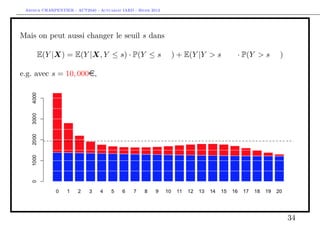
![Arthur CHARPENTIER - ACT2040 - Actuariat IARD - Hiver 2013
Prise en compte des gros sinistres
Reste à combiner les modèles, e.g.
E(Y |X) = E(Y |X, Y ≤ s) · P(Y ≤ s|X) + E(Y |Y > s, X) · P(Y > s|X)
> indice = which(couts$cout>s)
> mean(couts$cout[indice])
[1] 34471.59
> prime = ypA*ypC + ypB*(1-ypC))
30](https://image.slidesharecdn.com/slides-2040-6-130215130733-phpapp01/85/Slides-2040-6-30-320.jpg)
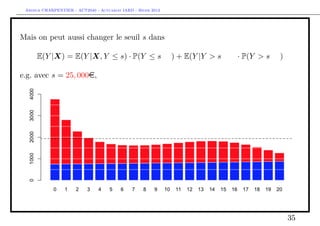
![Arthur CHARPENTIER - ACT2040 - Actuariat IARD - Hiver 2013
ou, e.g.
E(Y |X) = E(Y |X, Y ≤ s) · P(Y ≤ s|X) + E(Y |Y > s, X) · P(Y > s|X)
> indice = which(couts$cout>s)
> mean(couts$cout[indice])
[1] 34471.59
> prime = ypA*ypC + ypB2*(1-ypC))
32](https://image.slidesharecdn.com/slides-2040-6-130215130733-phpapp01/85/Slides-2040-6-32-320.jpg)
![Arthur CHARPENTIER - ACT2040 - Actuariat IARD - Hiver 2013
voire e.g.
E(Y |X) = E(Y |X, Y ≤ s) · P(Y ≤ s|X) + E(Y |Y > s, X) · P(Y > s|X)
> indice = which(couts$cout>s)
> mean(couts$cout[indice])
[1] 34471.59
> prime = ypA*ypC + ypB2*(1-ypC))
33](https://image.slidesharecdn.com/slides-2040-6-130215130733-phpapp01/85/Slides-2040-6-33-320.jpg)
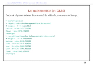
![Arthur CHARPENTIER - ACT2040 - Actuariat IARD - Hiver 2013
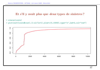
Et s’il y avait plus que deux types de sinistres ?
On peut considérer un mélange de trois lois,
f (y) = p1 f1 (x) + p2 δκ (x) + p3 f3 (x), ∀y ∈ R+
avec
1. une loi exponentielle pour f1
2. une masse de Dirac en κ (i.e. un coût fixe) pour f2
3. une loi lognormale (décallée) pour f3
> I1=which(couts$cout<1120)
> I2=which((couts$cout>=1120)&(couts$cout<1220))
> I3=which(couts$cout>=1220)
> (p1=length(I1)/nrow(couts))
[1] 0.3284823
> (p2=length(I2)/nrow(couts))
[1] 0.4152807
> (p3=length(I3)/nrow(couts))
38](https://image.slidesharecdn.com/slides-2040-6-130215130733-phpapp01/85/Slides-2040-6-38-320.jpg)
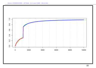
![Arthur CHARPENTIER - ACT2040 - Actuariat IARD - Hiver 2013
[1] 0.256237
> X=couts$cout
> (kappa=mean(X[I2]))
[1] 1171.998
> X0=X[I3]-kappa
> u=seq(0,10000,by=20)
> F1=pexp(u,1/mean(X[I1]))
> F2= (u>kappa)
> F3=plnorm(u-kappa,mean(log(X0)),sd(log(X0))) * (u>kappa)
> F=F1*p1+F2*p2+F3*p3
> lines(u,F,col="blue")
39](https://image.slidesharecdn.com/slides-2040-6-130215130733-phpapp01/85/Slides-2040-6-39-320.jpg)
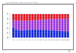
![Arthur CHARPENTIER - ACT2040 - Actuariat IARD - Hiver 2013
Prise en compte des coûts fixes en tarification
Comme pour les gros sinistres, on peut utiliser ce découpage pour calculer E(Y ),
ou E(Y |X). Ici,
E(Y |X) = E(Y |X, Y ≤ s1 ) ·P(Y ≤ s1 |X)
A D,π1 (X)
+E(Y |Y ∈ (s1 , s2 ], X) · P(Y ∈ (s1 , s2 ]|X)
B D,π2 (X)
+E(Y |Y > s2 , X) · P(Y > s2 |X)
C D,π3 (X)
Les paramètres du mélange, (π1 (X), π2 (X), π3 (X)) peuvent être associés à une
loi multinomiale de dimension 3.
41](https://image.slidesharecdn.com/slides-2040-6-130215130733-phpapp01/85/Slides-2040-6-41-320.jpg)
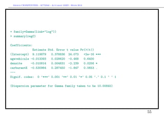
![Arthur CHARPENTIER - ACT2040 - Actuariat IARD - Hiver 2013
Estimate Std. Error z value Pr(>|z|)
(Intercept) 6.0600491 0.1005279 60.282 <2e-16 ***
agevehicule 0.0003965 0.0070390 0.056 0.955
densite 0.0014085 0.0013541 1.040 0.298
carburantE -0.0751446 0.0806202 -0.932 0.351
---
Signif. codes: 0 ’***’ 0.001 ’**’ 0.01 ’*’ 0.05 ’.’ 0.1 ’ ’ 1
(Dispersion parameter for Gamma family taken to be 1)
Pour B, on va garder l’idée d’une masse de Dirac en
> mean(sousbaseB$cout)
[1] 1171.998
(qui semble correspondre à un coût fixe.
Enfin, pour C, on peut tenter une loi Gamma ou lognormale décallée,
> k=mean(sousbaseB$cout)
> regC=glm((cout-k)~agevehicule+densite+carburant,data=sousbaseC,
54](https://image.slidesharecdn.com/slides-2040-6-130215130733-phpapp01/85/Slides-2040-6-54-320.jpg)

Le document discute de la modélisation des coûts individuels de sinistres en actuariat, en se concentrant sur les modèles de régression tels que la régression log-poisson, gamma, lognormale et inverse gaussienne. Il présente des exemples de calculs et les propriétés de différents modèles de distribution, y compris les implications des choix de fonction lien et des variables explicatives. La conclusion souligne l'importance de choisir le modèle adapté en fonction des caractéristiques des données de sinistres.


