Télécharger pour lire hors ligne


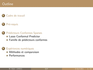
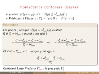
![Pr´diction Conforme :
e Vovk et al. ’05
Notations :
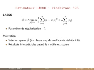
y ∈ R : valeur possible de ynew
|A| : cardinal de l’ensemble A
Score de Non-conformit´ α(y) = (α1 (y), . . . , αn (y), αnew (y))
e
αi (y) : similarit´ entre (xnew , y) et (xi , yi )
e
information relative : p-value
1
p(y) = | {i ∈ {1, . . . , n, new} : αnew (y) ≤ αi (y)} |
n+1
1
p(y) ∈ [ n+1 ; 1]
plus p(y) est petite, moins la paire test´e (xnew , y) est vraisemblable
e
(ce choix fait de y une valeur aberrante lorsqu’elle est combin´e avec
e
xnew )
Pr´dicteur Conforme Γε : valeurs y ∈ R telle que p(y) > ε.
e
M. Hebiri (UMLV) SCP 8 Avril 2011 6 / 21](https://image.slidesharecdn.com/scp-110411045534-phpapp01/85/Prediction-conforme-sparse-6-320.jpg)
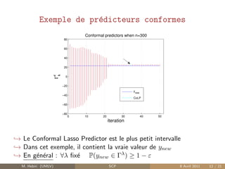
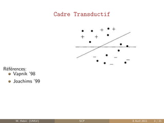
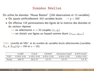
![Validit´
e
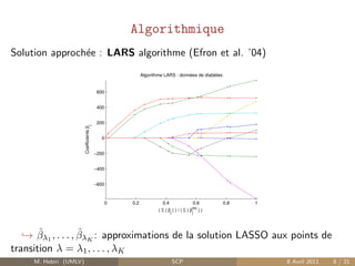
Table: Contrˆle de VALε
o
Exemple[n/σ] CoRP CoLP CoLaRP CENeP
Ex (a)[300/1] 0.90± 0.02 0.88± 0.02 0.85± 0.02 0.88± 0.02
Ex (a)[300/7] 0.89± 0.02 0.91± 0.02 0.89± 0.02 0.90± 0.02
Ex (a)[300/15] 0.89± 0.02 0.89 ± 0.02 0.88± 0.02 0.89± 0.02
Ex (b)[300/1] 0.90± 0.02 0.88± 0.02 0.87± 0.02 0.87± 0.02
Ex (c)[300/1] 0.90± 0.02 0.90± 0.02 0.89± 0.02 0.90± 0.02
Ex (d)[300/1] 0.89± 0.02 0.90± 0.02 0.90± 0.02 0.90± 0.02
Ex (a)[50/3] 0.89± 0.02 0.67± 0.03 0.41± 0.03 0.79± 0.02
Ex (a)[20/3] 0.86± 0.02 0.60± 0.03 0.30± 0.03 0.69± 0.03
Exemple[n/σ] CoRP CoLP Stopped-CoLP 2-PN-CoLP
Ex (a)[50/7] 0.85± 0.02 0.62± 0.03 0.82± 0.02 0.88± 0.02
Ex (b)[50/1] 0.88± 0.02 0.56± 0.03 0.82± 0.02 0.91 ± 0.02
Ex (c)[20/15] 0.88± 0.02 0.61± 0.03 0.77± 0.03 0.90± 0.02
Ex (d)[20/1] 0.90± 0.02 0.60± 0.03 0.79± 0.02 0.89± 0.02
M. Hebiri (UMLV) SCP 8 Avril 2011 16 / 21](https://image.slidesharecdn.com/scp-110411045534-phpapp01/85/Prediction-conforme-sparse-16-320.jpg)
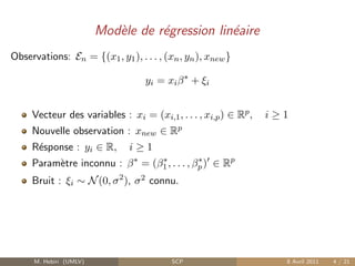
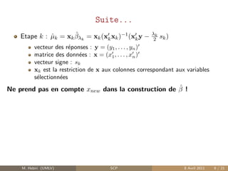
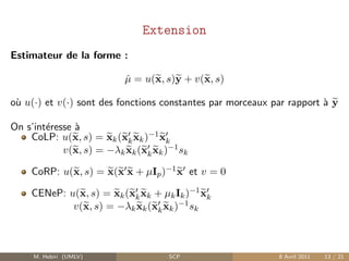
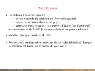
![S´lection de variables :
e Exemple(b)[300/5]
50 50
45 45
40 40
35 35
30 30
Iteration
Iteration
25 25
20 20
CoLP
15 CoRLaP 15 CENeP
Lasso Elastic−Net
10 10
5 5
0 0
0 5 10 15 20 25 30 35 40 45 50 0 5 10 15 20 25 30 35 40 45 50
Variable index Variable index
M. Hebiri (UMLV) SCP 8 Avril 2011 17 / 21](https://image.slidesharecdn.com/scp-110411045534-phpapp01/85/Prediction-conforme-sparse-17-320.jpg)
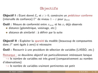
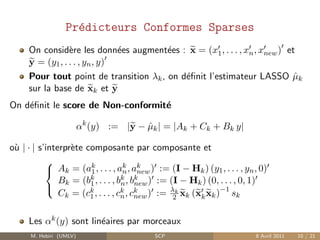
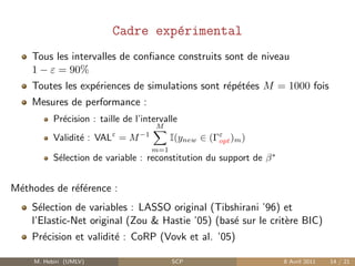
![Pr´cision :
e Exemple(b)[n/5]
4
90 x 10
2.5
Selected predictor
80
Selected predictor
Failed predictor
70 2
60
Intervals sizes
Intervals sizes
1.5
50
40
1
30
20
0.5
10
0 0
0 5 10 15 20 25 30 35 40 45 50 0 50 100 150 200 250 300 350 400
Iteration Iteration
M. Hebiri (UMLV) SCP 8 Avril 2011 18 / 21](https://image.slidesharecdn.com/scp-110411045534-phpapp01/85/Prediction-conforme-sparse-18-320.jpg)


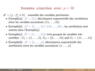
Ce document présente une étude sur les prédicteurs conformes sparses, mettant l'accent sur l'utilisation du lasso comme outil de sélection des variables dans un cadre de régression linéaire. Il décrit des méthodes expérimentales pour la validation de ces prédicteurs, ainsi que des résultats de performance sur des données simulées et réelles. Les conclusions soulignent l'efficacité des prédicteurs conformes sparses, notamment lorsque le nombre de variables dépasse le nombre d'observations.


