O.Venard - ESIEE/SIGTEL- 2005 2
Transformée en Z
Cas continu :
( )
( ) ( )
ds t
e t s t RC
dt
= +
( )
( )
( )
S p
H p
E p
= 2
( ) ( ) p j f
H f H p π
=
=
discrètisation :
[ ] [ ]
[ ] ( )
1
e e
e e
e
s nT s n T
e nT s nT RC
T
⎡ ⎤
− −
⎣ ⎦
= +
( )
( )
( )
S z
H z
E z
= 2 f
("f ") ( ) j
z e
H H z π
=
=
3.
O.Venard - ESIEE/SIGTEL- 2005 3
Transformée de Laplace d’un signal échantillonné :
( ) ( ) ( ) ( )
avec
pt
e e e e
X p x t e dt x t x nT
+∞
−
−∞
= =
∫
( ) [ ] e
npT
e e
n
X p x n e
+∞
−
=−∞
= ∑
4.
O.Venard - ESIEE/SIGTEL- 2005 4
Transformée en Z
( ) [ ] n
n
X z x n z
+∞
−
=−∞
= ∑
( ) [ ] [ ]
= avec
e e
npT pT
n
e e e
n n
X p x n e x n z z e
+∞ +∞
− −
=−∞ =−∞
= =
∑ ∑
O.Venard - ESIEE/SIGTEL- 2005 6
Systèmes LIT
Stabilité
Fonction de transfert discrète :
( ) [ ] n
n
H z h n z
+∞
−
=−∞
= ∑
[ ]
0
<
n
h n
+∞
=
∞
∑
Causalité
[ ] [ ] [ ]
0
m
y n h m x n m
+∞
=
= −
∑
( ) [ ]
0
n
n
H z h n z
+∞
−
=
= ∑
7.
O.Venard - ESIEE/SIGTEL- 2005 7
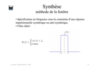
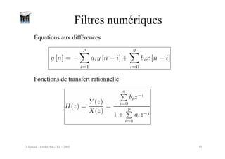
Filtres numériques
Équations aux différences
Fonctions de transfert rationnelle
8.
O.Venard - ESIEE/SIGTEL- 2005 8
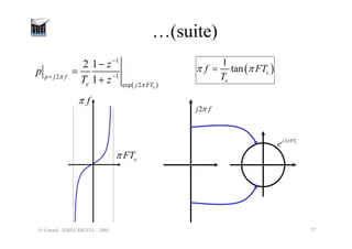
…(suite)
( )
( )
( )
( )
1
0 1
1
1 1
1
( )
1 1
q
q
i
i
i
i i
p p
i
i i
i i
z
b z
N z
H z
D z
a z z
β
α
−
−
= =
− −
= =
−
= = =
+ −
∑ ∏
∑ ∏
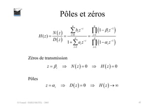
Pôles et zéros
( ) ( )
0 0
i
z N z H z
β
= ⇒ = ⇒ =
Zéros de transmission
Pôles
( ) ( )
0
i
z D z H z
α
= ⇒ = ⇒ → ∞
stable si 1
i
α
⎡ ⎤
<
⎣ ⎦
9.
O.Venard - ESIEE/SIGTEL- 2005 9
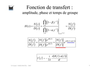
Fonction de transfert :
amplitude, phase et temps de groupe
( )
( )
( )
( )
( )
( )
2
1
1
1
1
1
( )
1
j f
q
i
i
p
i
i z e
z
N z N f
H z
D z D f
z
π
β
α
−
=
−
= =
−
= = =
−
∏
∏
( )
( )
( ) ( )
( ) ( )
( )
( )
( ) ( )
( )
j f
j f f
j f
N f e N f
N f
e
D f D f
D f e
θ
θ ϕ
ϕ
−
= =
( )
( ) ( )
( )
1
2
d f f
T f
df
θ ϕ
π
−
= −
10.
O.Venard - ESIEE/SIGTEL- 2005 10
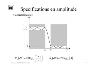
Spécifications en amplitude
Gabarit (linéaire)
( ) 10
1
20log
1
p
e
R dB
e
+
⎛ ⎞
= ⎜ ⎟
−
⎝ ⎠
( ) ( )
10
20log
s
R dB A
=
O.Venard - ESIEE/SIGTEL- 2005 12
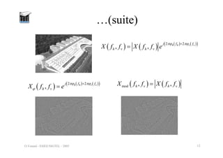
…(suite)
( ) ( ) ( ) ( )
( )
2 2
, , h h v v
j f f
h v h v
X f f X f f e
πϕ πϕ
+
=
( ) ( ) ( )
( )
2 2
, h h v v
j f f
h v
X f f e
πϕ πϕ
ϕ
+
= ( ) ( )
mod , ,
h v h v
X f f X f f
=
O.Venard - ESIEE/SIGTEL- 2005 15
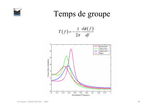
…(suite)
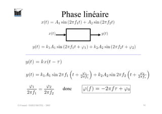
Temps de groupe
( ) ( )
0
2
1
2
d f
T f
df
π τ ϕ
τ
π
− +
= − =
Condition
• h(t) doit être symétrique ou antisymétrique
• Non réalisable avec les filtres analogiques
16.
O.Venard - ESIEE/SIGTEL- 2005 16
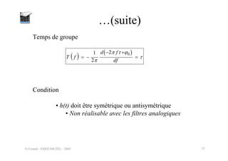
Synthèse
méthode de la fenêtre
• Spécification en fréquence sous la contrainte d’une réponse
impulsionnelle symétrique ou anti-symétrique.
• Filtre idéal :
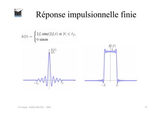
17.
O.Venard - ESIEE/SIGTEL- 2005 17
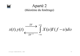
Aparté 1
(Fonctions rectangle et sinus cardinal)
( )
1 if
2
0 else.
c
c
f
f
rect f f
⎧ <
= ⎨
⎩
sin( 2 )
2 sinc(2 ) 2
2
c
c c c
c
f t
f f t f
f t
π
π
=
1
TF−
⎯⎯⎯
→
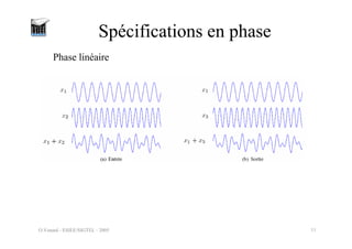
O.Venard - ESIEE/SIGTEL- 2005 24
Phase
Système causal
( ) ( ) ( ) ( )
exp 2
TF
f f
h t t t H f j f t
δ π
∗ − ⎯⎯
→ −
( ) f
T f t
=
25.
O.Venard - ESIEE/SIGTEL- 2005 25
Phase (cas discret)
Soit h[n] = h(nTe) et LTe = tf , alors,
[ ] [ ] [ ] exp 2
TFD
e
k
h n n L H k j L
F
δ π
⎛ ⎞
∗ − ⎯⎯⎯
→ −
⎜ ⎟
⎝ ⎠
Causalité :
N coefficients :
1
2
N
L
−
=
2LTe
O.Venard - ESIEE/SIGTEL- 2005 28
Réponse impulsionnelle, fonction de transfert,
stabilité et équation aux différences
Réponse impulsionnelle : h[n]
Fonction de transfert :
( )
( )
( )
[ ]
1
0
N
k
k
Y z
H z h k z
X z
−
−
=
= = ∑
Equation aux différences :
( ) [ ] [ ]
( )
( )
( )
1
0 1
N
k k
k k
N z N z
H z h k z h k z
D z
+∞ −
− −
=−∞ =
= = = =
∑ ∑
( ) [ ] ( ) ( )
1 1
0 0
N N
k k
k
k k
Y z h k X z z b X z z
− −
− −
= =
= =
∑ ∑
[ ] [ ]
1
0
N
k
k
y n b x n k
−
=
= −
∑
O.Venard - ESIEE/SIGTEL- 2005 35
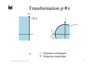
Transformation pÆz
2
j f
π
+∞
−∞
j
2
e
F
2
e
F
−
2 e
j FT
e π
f : fréquence analogique
F : fréquence numérique
36.
O.Venard - ESIEE/SIGTEL- 2005 36
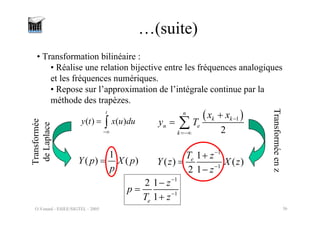
…(suite)
• Transformation bilinéaire :
• Réalise une relation bijective entre les fréquences analogiques
et les fréquences numériques.
• Repose sur l’approximation de l’intégrale continue par la
méthode des trapèzes.
( ) ( )
t
y t x u du
−∞
= ∫
( )
1
2
n
k k
n e
k
x x
y T −
=−∞
+
= ∑
1
( ) ( )
Y p X p
p
=
1
1
1
( ) ( )
2 1
e
T z
Y z X z
z
−
−
+
=
−
1
1
2 1
1
e
z
p
T z
−
−
−
=
+
Transformée
de
Laplace
Transformée
en
z
37.
O.Venard - ESIEE/SIGTEL- 2005 37
…(suite)
( )
1
1
2
exp 2
2 1
1
e
p j f
e j FT
z
p
T z
π
π
−
−
=
−
=
+
( )
1
tan e
e
f FT
T
π π
=
2
j f
π
2 e
j FT
e π
e
FT
π
f
π
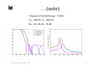
O.Venard - ESIEE/SIGTEL- 2005 39
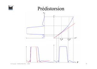
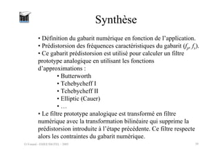
Synthèse
• Définition du gabarit numérique en fonction de l’application.
• Prédistorsion des fréquences caractéristiques du gabarit (fp, fs).
• Ce gabarit prédistorsion est utilisé pour calculer un filtre
prototype analogique en utilisant les fonctions
d’approximations :
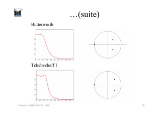
• Butterworth
• Tchebycheff I
• Tchebycheff II
• Elliptic (Cauer)
• …
• Le filtre prototype analogique est transformé en filtre
numérique avec la transformation bilinéaire qui supprime la
prédistorsion introduite à l’étape précédente. Ce filtre respecte
alors les contraintes du gabarit numérique.
40.
O.Venard - ESIEE/SIGTEL- 2005 40
Filtres numériques
Équations aux différences
Fonctions de transfert rationnelle
41.
O.Venard - ESIEE/SIGTEL- 2005 41
Caractéristiques des filtres RII
2
2
1
( )
1
N
c
H f
f
f
=
⎛ ⎞
+ ⎜ ⎟
⎝ ⎠
• Filtres de Butterworth
• Défini par son ordre N et sa fréquence de
coupure fc.
• Fonction de transfert en module monotone.
% Butterworth filter
% sampling frequency : 16 kHz
% Fp : 1800 Hz
% Fa : 4000 Hz
% Rp : 0.01 dB % Ra : 50 dB
[N, Wn]= buttord(1800/8000,4000/8000,0.01,50);
[B,A] = butter(N,Wn);
H=freqz(B,A);
plot(linspace(0,1,512),abs(H))
42.
O.Venard - ESIEE/SIGTEL- 2005 42
…(suite)
• Filtres de Tchebycheff I
2
2 2
1
( )
1 N
p
H f
f
T
f
ε
=
⎛ ⎞
+ ⎜ ⎟
⎜ ⎟
⎝ ⎠
• Défini par son ordre N et la fréquence
délimitant la bande passante fp et ε l’ondulation
en bande passante.
• Ondulation en bande passante et monotone en
bande atténuée.
TN( ) est un polynome de Tchebycheff d’ordre N
% Chebyshev I filter
% sampling frequency : 16 kHz
% Fp : 1800 Hz
% Fa : 4000 Hz
% Rp : 0.01 dB
% Ra : 50 dB
[N, Wn] =
cheb1ord(1800/8000,4000/8000,0.01,50); [B,A] =
cheby1(N,0.01,Wn);
H=freqz(B,A);
plot(linspace(0,1,512),abs(H))
43.
O.Venard - ESIEE/SIGTEL- 2005 43
2
2 2
1
( ) 1
1 s
N
H f
f
T
f
ε
= −
⎛ ⎞
+ ⎜ ⎟
⎝ ⎠
…(suite)
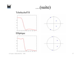
• Filtres de Tchebycheff II
• Défini par son ordre N, la fréquence délimitant
la bande atténuée fs et l’atténuation ε.
• Monotone en bande passante et ondulation en
bande atténuée.
TN( ) est un polynome de Tchebycheff d’ordre N
% Chebyshev II filter
% sampling frequency : 16 kHz
% Fp : 1800 Hz
% Fa : 4000 Hz
% Rp : 0.01 dB
% Ra : 50 dB
[N, Wn] =
cheb2ord(1800/8000,4000/8000,0.01,50); [B,A] =
cheby2(N,50,Wn);
H=freqz(B,A);
plot(linspace(0,1,512),abs(H))
44.
O.Venard - ESIEE/SIGTEL- 2005 44
2
2 2
1
( )
1 N
p s
H f
f
R
f f
ε
=
⎛ ⎞
⎜ ⎟
+
⎜ ⎟
⎝ ⎠
…(suite)
• Filtres elliptique
• Défini par son ordre N et la fréquence
délimitant la bande atténuée fs, la fréquence
délimitant la bande passante fp et ε l’atténuation
et l’ondulation en bande passante.
• Ondulation en bande passante et ondulation en
bande atténuée.
RN( ) est un polynome rationnel de Tchebycheff d’ordre N
% Elliptic filter
% sampling frequency : 16 kHz
% Fp : 1800 Hz
% Fa : 4000 Hz
% Rp : 0.01 dB % Ra : 50 dB
[N, Wn] =
ellipord(1800/8000,4000/8000,0.01,50);
[B,A] = ellip(N,0.01,50,Wn);
H=freqz(B,A);
plot(linspace(0,1,512),abs(H))
45.
O.Venard - ESIEE/SIGTEL- 2005 45
Pôles et zéros
( )
( )
( )
( )
1
0 1
1
1 1
1
( )
1 1
q
q
i
i
i
i i
p p
i
i i
i i
z
b z
N z
H z
D z
a z z
β
α
−
−
= =
− −
= =
−
= = =
+ −
∑ ∏
∑ ∏
( ) ( )
0 0
i
z N z H z
β
= ⇒ = ⇒ =
Zéros de transmission
Pôles
( ) ( )
0
i
z D z H z
α
= ⇒ = ⇒ → ∞
O.Venard - ESIEE/SIGTEL- 2005 50
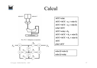
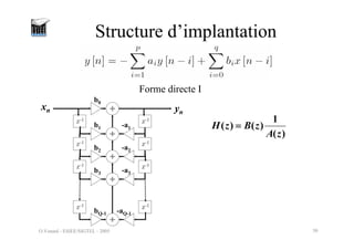
Structure d’implantation
z-1
z-1
z-1
z-1
z-1
z-1
z-1 z-1
b1
b0
b2
b3
bQ-1
-a1
-a2
-a3
-aQ-1
xn yn
)
(
1
)
(
)
(
z
A
z
B
z
H =
Forme directe I
51.
O.Venard - ESIEE/SIGTEL- 2005 51
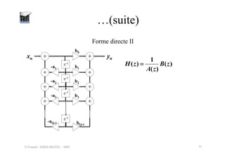
…(suite)
z
z-
-1
1
z
z-
-1
1
z
z-
-1
1
z
z-
-1
1
b1
b0
b2
b3
bQ-1
-a1
-a2
-a3
-aQ-1
yn
xn
)
(
)
(
1
)
( z
B
z
A
z
H =
Forme directe II
52.
O.Venard - ESIEE/SIGTEL- 2005 52
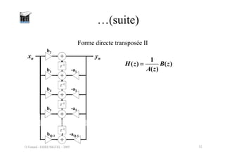
…(suite)
b2
b3
bQ-1
-a1
-a2
-a3
-aQ-1
xn
z-1
z-1
b1
z-1
b2
z-1
yn
)
(
)
(
1
)
( z
B
z
A
z
H =
Forme directe transposée II
53.
O.Venard - ESIEE/SIGTEL- 2005 53
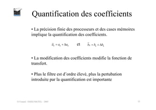
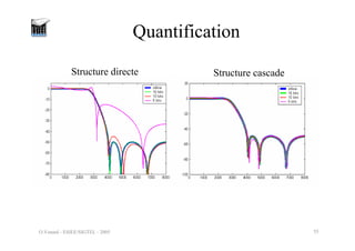
Quantification des coefficients
• La précision finie des processeurs et des cases mémoires
implique la quantification des coefficients.
k k k
a a a
= + Δ et k k k
b b b
= + Δ
• La modification des coefficients modifie la fonction de
transfert.
• Plus le filtre est d’ordre élevé, plus la pertubation
introduite par la quantification est importante
54.
O.Venard - ESIEE/SIGTEL- 2005 54
…(suite)
• sensibilité des coefficients à la quantification Æ cellules
d’ordre 2
2
2
1
1
1
1
0
1 −
−
−
+
+
+
z
a
z
a
z
b
b
2
2
1
1
1
1
0
1 −
−
−
+
+
+
z
a
z
a
z
b
b
xn yn
Décomposition en éléments simples
∑
−
=
−
−
−
+
+
+
+
=
1
0
2
2
1
1
1
1
0
0
1
)
(
)
( N
i i
i
i
i
z
a
z
a
z
b
b
c
z
A
z
B
c0
Structure parallèle Structure cascade
2
2
1
1
2
2
1
1
0
1 −
−
−
−
+
+
+
+
z
a
z
a
z
b
z
b
b
2
2
1
1
2
2
1
1
0
1 −
−
−
−
+
+
+
+
z
a
z
a
z
b
z
b
b
x
xn
n y
yn
n
Factorisation spectrale
∏
−
=
−
−
−
−
+
+
+
+
=
1
0
2
2
1
1
2
2
1
1
0
1
1
)
(
)
( N
i i
i
i
i
z
a
z
a
z
b
z
b
b
z
A
z
B
O.Venard - ESIEE/SIGTEL- 2005 56
Factorisation spectrale
%calcul des racines
P=roots(A)
Z=roots(B)
% fabrication des polynomes d’ordre 2
%à partir des racines complexes conjuguées
A1=poly(P(1:2))
B1=poly(Z(3:4))
A2=poly(P(3:4))
B2=poly(Z(5:6))
A3=poly(P(5:6))
B3=poly(Z(1:2))
% Cela peut être fait automatiquement par la fonction matlab
% [sos,g]=tf2sos(B,A);
1
1
2
2
3
3
![O.Venard - ESIEE/SIGTEL - 2005 2
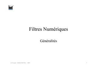
Transformée en Z
Cas continu :
( )
( ) ( )
ds t
e t s t RC
dt
= +
( )
( )
( )
S p
H p
E p
= 2
( ) ( ) p j f
H f H p π
=
=
discrètisation :
[ ] [ ]
[ ] ( )
1
e e
e e
e
s nT s n T
e nT s nT RC
T
⎡ ⎤
− −
⎣ ⎦
= +
( )
( )
( )
S z
H z
E z
= 2 f
("f ") ( ) j
z e
H H z π
=
=](https://image.slidesharecdn.com/filtresnumeriques-251128185345-a6bb208c/85/FiltresNumeriques-pdf-2-320.jpg)
![O.Venard - ESIEE/SIGTEL - 2005 3
Transformée de Laplace d’un signal échantillonné :
( ) ( ) ( ) ( )
avec
pt
e e e e
X p x t e dt x t x nT
+∞
−
−∞
= =
∫
( ) [ ] e
npT
e e
n
X p x n e
+∞
−
=−∞
= ∑](https://image.slidesharecdn.com/filtresnumeriques-251128185345-a6bb208c/85/FiltresNumeriques-pdf-3-320.jpg)
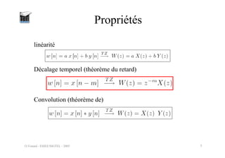
![O.Venard - ESIEE/SIGTEL - 2005 4
Transformée en Z
( ) [ ] n
n
X z x n z
+∞
−
=−∞
= ∑
( ) [ ] [ ]
= avec
e e
npT pT
n
e e e
n n
X p x n e x n z z e
+∞ +∞
− −
=−∞ =−∞
= =
∑ ∑](https://image.slidesharecdn.com/filtresnumeriques-251128185345-a6bb208c/85/FiltresNumeriques-pdf-4-320.jpg)
![O.Venard - ESIEE/SIGTEL - 2005 6
Systèmes LIT
Stabilité
Fonction de transfert discrète :
( ) [ ] n
n
H z h n z
+∞
−
=−∞
= ∑
[ ]
0
<
n
h n
+∞
=
∞
∑
Causalité
[ ] [ ] [ ]
0
m
y n h m x n m
+∞
=
= −
∑
( ) [ ]
0
n
n
H z h n z
+∞
−
=
= ∑](https://image.slidesharecdn.com/filtresnumeriques-251128185345-a6bb208c/85/FiltresNumeriques-pdf-6-320.jpg)


![O.Venard - ESIEE/SIGTEL - 2005 25
Phase (cas discret)
Soit h[n] = h(nTe) et LTe = tf , alors,
[ ] [ ] [ ] exp 2
TFD
e
k
h n n L H k j L
F
δ π
⎛ ⎞
∗ − ⎯⎯⎯
→ −
⎜ ⎟
⎝ ⎠
Causalité :
N coefficients :
1
2
N
L
−
=
2LTe](https://image.slidesharecdn.com/filtresnumeriques-251128185345-a6bb208c/85/FiltresNumeriques-pdf-25-320.jpg)
![O.Venard - ESIEE/SIGTEL - 2005 28
Réponse impulsionnelle, fonction de transfert,
stabilité et équation aux différences
Réponse impulsionnelle : h[n]
Fonction de transfert :
( )
( )
( )
[ ]
1
0
N
k
k
Y z
H z h k z
X z
−
−
=
= = ∑
Equation aux différences :
( ) [ ] [ ]
( )
( )
( )
1
0 1
N
k k
k k
N z N z
H z h k z h k z
D z
+∞ −
− −
=−∞ =
= = = =
∑ ∑
( ) [ ] ( ) ( )
1 1
0 0
N N
k k
k
k k
Y z h k X z z b X z z
− −
− −
= =
= =
∑ ∑
[ ] [ ]
1
0
N
k
k
y n b x n k
−
=
= −
∑](https://image.slidesharecdn.com/filtresnumeriques-251128185345-a6bb208c/85/FiltresNumeriques-pdf-28-320.jpg)
![O.Venard - ESIEE/SIGTEL - 2005 29
Implantation [ ] [ ]
1
0
N
k
k
y n b x n k
−
=
= −
∑](https://image.slidesharecdn.com/filtresnumeriques-251128185345-a6bb208c/85/FiltresNumeriques-pdf-29-320.jpg)
![O.Venard - ESIEE/SIGTEL - 2005 30
…(suite)
[ ] [ ]
1
0
N
k
k
y n b x n k
−
=
= −
∑](https://image.slidesharecdn.com/filtresnumeriques-251128185345-a6bb208c/85/FiltresNumeriques-pdf-30-320.jpg)

![O.Venard - ESIEE/SIGTEL - 2005 41
Caractéristiques des filtres RII
2
2
1
( )
1
N
c
H f
f
f
=
⎛ ⎞
+ ⎜ ⎟
⎝ ⎠
• Filtres de Butterworth
• Défini par son ordre N et sa fréquence de
coupure fc.
• Fonction de transfert en module monotone.
% Butterworth filter
% sampling frequency : 16 kHz
% Fp : 1800 Hz
% Fa : 4000 Hz
% Rp : 0.01 dB % Ra : 50 dB
[N, Wn]= buttord(1800/8000,4000/8000,0.01,50);
[B,A] = butter(N,Wn);
H=freqz(B,A);
plot(linspace(0,1,512),abs(H))](https://image.slidesharecdn.com/filtresnumeriques-251128185345-a6bb208c/85/FiltresNumeriques-pdf-41-320.jpg)
![O.Venard - ESIEE/SIGTEL - 2005 42
…(suite)
• Filtres de Tchebycheff I
2
2 2
1
( )
1 N
p
H f
f
T
f
ε
=
⎛ ⎞
+ ⎜ ⎟
⎜ ⎟
⎝ ⎠
• Défini par son ordre N et la fréquence
délimitant la bande passante fp et ε l’ondulation
en bande passante.
• Ondulation en bande passante et monotone en
bande atténuée.
TN( ) est un polynome de Tchebycheff d’ordre N
% Chebyshev I filter
% sampling frequency : 16 kHz
% Fp : 1800 Hz
% Fa : 4000 Hz
% Rp : 0.01 dB
% Ra : 50 dB
[N, Wn] =
cheb1ord(1800/8000,4000/8000,0.01,50); [B,A] =
cheby1(N,0.01,Wn);
H=freqz(B,A);
plot(linspace(0,1,512),abs(H))](https://image.slidesharecdn.com/filtresnumeriques-251128185345-a6bb208c/85/FiltresNumeriques-pdf-42-320.jpg)
![O.Venard - ESIEE/SIGTEL - 2005 43
2
2 2
1
( ) 1
1 s
N
H f
f
T
f
ε
= −
⎛ ⎞
+ ⎜ ⎟
⎝ ⎠
…(suite)
• Filtres de Tchebycheff II
• Défini par son ordre N, la fréquence délimitant
la bande atténuée fs et l’atténuation ε.
• Monotone en bande passante et ondulation en
bande atténuée.
TN( ) est un polynome de Tchebycheff d’ordre N
% Chebyshev II filter
% sampling frequency : 16 kHz
% Fp : 1800 Hz
% Fa : 4000 Hz
% Rp : 0.01 dB
% Ra : 50 dB
[N, Wn] =
cheb2ord(1800/8000,4000/8000,0.01,50); [B,A] =
cheby2(N,50,Wn);
H=freqz(B,A);
plot(linspace(0,1,512),abs(H))](https://image.slidesharecdn.com/filtresnumeriques-251128185345-a6bb208c/85/FiltresNumeriques-pdf-43-320.jpg)
![O.Venard - ESIEE/SIGTEL - 2005 44
2
2 2
1
( )
1 N
p s
H f
f
R
f f
ε
=
⎛ ⎞
⎜ ⎟
+
⎜ ⎟
⎝ ⎠
…(suite)
• Filtres elliptique
• Défini par son ordre N et la fréquence
délimitant la bande atténuée fs, la fréquence
délimitant la bande passante fp et ε l’atténuation
et l’ondulation en bande passante.
• Ondulation en bande passante et ondulation en
bande atténuée.
RN( ) est un polynome rationnel de Tchebycheff d’ordre N
% Elliptic filter
% sampling frequency : 16 kHz
% Fp : 1800 Hz
% Fa : 4000 Hz
% Rp : 0.01 dB % Ra : 50 dB
[N, Wn] =
ellipord(1800/8000,4000/8000,0.01,50);
[B,A] = ellip(N,0.01,50,Wn);
H=freqz(B,A);
plot(linspace(0,1,512),abs(H))](https://image.slidesharecdn.com/filtresnumeriques-251128185345-a6bb208c/85/FiltresNumeriques-pdf-44-320.jpg)

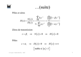
![O.Venard - ESIEE/SIGTEL - 2005 56
Factorisation spectrale
%calcul des racines
P=roots(A)
Z=roots(B)
% fabrication des polynomes d’ordre 2
%à partir des racines complexes conjuguées
A1=poly(P(1:2))
B1=poly(Z(3:4))
A2=poly(P(3:4))
B2=poly(Z(5:6))
A3=poly(P(5:6))
B3=poly(Z(1:2))
% Cela peut être fait automatiquement par la fonction matlab
% [sos,g]=tf2sos(B,A);
1
1
2
2
3
3](https://image.slidesharecdn.com/filtresnumeriques-251128185345-a6bb208c/85/FiltresNumeriques-pdf-56-320.jpg)