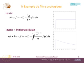
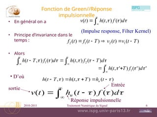
Le document aborde divers concepts fondamentaux du traitement numérique du signal, incluant les filtres analogiques, la convolution, la transformée de Laplace, et les propriétés des systèmes invariants. Il traite également des concepts avancés tels que la réponse impulsionnelle, les filtres linéaires, et la relation entrée-sortie. Enfin, le texte mentionne la stabilité des filtres et les caractéristiques de minimum de phase.

1. 2010-2011 Traitement Numérique du Signal 1
Université Paris 13
Traitement Numérique du Signal Master 1
1. Exemple de filtres analogiques
2. Principe d’invariance et réponse impulsionnelle
3. Propriétés du produit de convolution
4. Transformée de Laplace
5. Filtres et Fonction de transfert
6. Critère de stabilité, pôle, zéro
7. Filtre à phase linéaire
8. Schéma général

2. 2010-2011 Traitement Numérique du Signal 2
1/ Exemple de filtre analogique




t
d
f
m
t
v
f
v
m
0
)
(
1
)
( 









t t
m
d
f
m
e
t
v
f
v
v
m
0
)
(
)
(
)
( 





inertie
inertie + frottement fluide

3. 2010-2011 Traitement Numérique du Signal 3
Exemple de filtrages
Entrée
Réponse
impulsionnelle Sorties
t
t
t

4. 2010-2011 Traitement Numérique du Signal 4
Fonctionnement du produit de
convolution







t t
m
d
f
m
e
t
v
f
v
v
m
0
)
(
)
(
)
( 





h(t)
f(t)
v(t)

5. 2010-2011 Traitement Numérique du Signal 5
2/ Propriétés d’invariance pour un système
physique
Invariance par translation spatiale
Invariance dans le temps

6. 2010-2011 Traitement Numérique du Signal 6
Fonction de Green//Réponse
impulsionnelle
• En général on a
• Principe d’invariance dans le
temps :
• Alors




 

 d
f
t
h
t
v )
(
)
,
(
)
(
)
(
)
(
)
(
)
( 1
2
1
2 T
t
v
t
v
T
t
f
t
f 














 




 d
T
f
t
h
d
f
T
t
h )
(
)
,
(
)
(
)
,
( 2
1





 '
)
'
(
)
'
,
( 1 

 d
f
T
t
h
• D’où )
(
)
,
(
)
,
( 

 



 t
h
T
t
h
T
t
h u





 

 d
f
t
h
t
v u )
(
)
(
)
(
(Impulse response, Filter Kernel)
Entrée
sortie
Réponse impulsionnelle

7. 2010-2011 Traitement Numérique du Signal 7
3/ Propriétés du produit de convolution
Propriétés des filtres temps invariant
      
0
1
0
1 *
)
(
*
)
( t
t
x
h
t
x
h
t
t
x
t
x 




      )
(
*
)
(
*
)
(
*
)
(
)
(
)
( 2
1
2
1 t
x
h
t
x
h
t
x
h
t
x
t
x
t
x 




  )
(
ˆ
)
(
ˆ
)
(
ˆ
)
(
*
)
( f
X
f
H
f
Y
t
x
h
t
y 


  )
(
)
(
)
(
)
(
*
)
( p
X
p
H
p
Y
t
x
h
t
y 


     
t
x
h
t
x
h
t
x
t
x *
*
)
(
)
( 1
1 
 













 



)
(
)
(
)
( t
x
dt
t
h
t
y
Conservation de la moyenne
Invariance temporelle
Superposition des signaux
Réponse fréquentielle
Fonction de
transfert
Amplification des signaux
Conservation de la périodicité       
T
t
x
h
t
x
h
T
t
x
t
x 



 *
)
(
*
)
(
     
  )
(
*
*
)
(
)
(
*
)
(
),
(
*
)
( 1
2
1
2 t
x
h
h
t
z
t
x
h
t
y
t
y
h
t
z 



Filtres en cascade
)
(
)
(
ˆ
)
(
)
( 2
t
x
f
H
t
y
e
t
x ft
j


 
Réponse harmonique

8. 2010-2011 Traitement Numérique du Signal 8
4/ Transformée de Laplace




0
)
(
)
( dt
e
t
s
p
S pt





 dt
e
t
s
f
S ft
j 
2
)
(
)
(
ˆ
   
t
e
t
s at
[
,
0
[
1 


module
phase
p=j2f
a
p
p
S


1
)
(
signal causal
Re(p)
f
t

9. 2010-2011 Traitement Numérique du Signal 9
Propriétés de la transformée de Laplace
 
    
0
2
2
0
f
j
p
S
p
t
s
e
TL t
f
j




   
  
      
p
Y
p
X
p
t
t
x
t
x
TL 
2
1 *
  )
(
)
](
[ 0
0 p
S
e
p
t
t
s
TL pt



Décalage fréquentiel
      )
(
)
(
)
](
[
)
(
)
](
[ p
Y
p
X
f
t
y
t
x
TL
p
aS
f
t
as
TL 



 
  
f
j
p
j
f
j
p
j
f
t
f
TF
f
j
p
f
j
p
f
t
f
TL
p
p
t
TL
p
t
TL R
R
R







2
1
2
1
2
1
2
1
)
](
1
)
2
[sin(
2
1
2
1
2
1
2
1
)
](
1
)
2
[cos(
1
1
1
)
)](
(
[ 0
0









 


    )
(
)
(
)
(
1
)
(
0
p
pS
p
s
d
d
TL
p
S
p
p
d
s
TL
t
t















 




)
(
)
( ap
aS
p
a
t
s
TL 












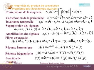
Retard=>déphasage
Linéarité
Dilatation/concentration
Intégration/dérivation
Produit de convolution/produit
Sinusoïdes=>hyperboles

10. 2010-2011 Traitement Numérique du Signal 10
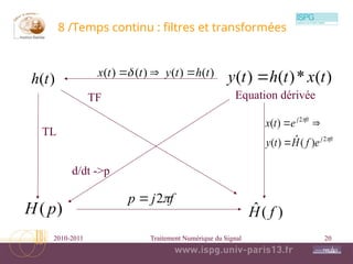
5/ Filtrage
 
)
(
)
( t
t
h 


    )
(
*
)
(
)
(
)
(
)
(
)
(
)
( t
u
t
t
t
y
t
t
u
t
y 





 
)
(
1 [
,
0
[ t


    )
(
*
)
(
)
(
1
)
(
)
(
)
(
)
( [
,
0
[
0
t
u
t
t
t
z
d
t
u
t
z
t





 

    t
f
j
t
f
j
e
f
H
t
e 0
0 2
0
2 ˆ
)
( 



  )
(
ˆ
)
(
ˆ
)
(
ˆ
)
(
)
(
)
( f
U
f
H
f
Y
t
t
u
t
y 



[
,
] 



t
]
[
)
( h
TL
p
H 
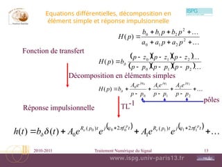
Réponse impulsionnelle
Réponse indicielle
Réponse harmonique ou réponse fréquentielle
Fonction de transfert
  )
(
)
(
)
(
)
(
)
(
)
( p
U
p
H
p
Y
t
t
u
t
y 



    )
(
ˆ f
h
TF
f
H 

11. 2010-2011 Traitement Numérique du Signal 11
Equations différentielles,
filtres linéaires et Réponses fréquentielles

 





 2
2
2
1
0
2
2
2
1
0
dt
x
d
b
dt
dx
b
x
b
dt
y
d
a
dt
dy
a
y
a









 2
2
1
0
2
2
1
0
)
(
)
(
)
(
p
a
p
a
a
p
b
p
b
b
p
X
p
Y
p
H
 
  







 2
2
1
0
2
2
1
0
2
2
2
2
)
(
ˆ
f
j
a
f
j
a
a
f
j
b
f
j
b
b
f
H




    )
(
)
( 2
2
1
0
2
2
1
0 p
X
p
b
p
b
b
p
Y
p
a
p
a
a 
 






Relation entrée-sortie
TL
Fonction de transfert
Réponse fréquentielle
p opérateur de dérivation

12. 2010-2011 Traitement Numérique du Signal 12
Pôles, zéros et allure de la réponse fréquentielle

 





 2
2
2
1
0
2
2
2
1
0
dt
x
d
b
dt
dx
b
x
b
dt
y
d
a
dt
dy
a
y
a









 2
2
1
0
2
2
1
0
)
(
)
(
)
(
p
a
p
a
a
p
b
p
b
b
p
X
p
Y
p
H
   
   
  









 
z
e
z
e
b f
f
j
z
R
f
f
j
z
R
f
H 1
1
0
0
0 2
)
(
arg
2
)
(
arg
1
)
(
ˆ
arg 

 
 
   
  








 p
e
p
e f
f
j
p
R
f
f
j
p
R 1
1
0
0 2
)
(
arg
2
)
(
arg 

   
   

2
1
0
2
1
0
)
(
p
p
p
p
p
p
z
p
z
p
z
p
b
p
H






 
           
           

2
2
2
2
2
1
2
2
1
2
0
2
2
0
2
2
2
2
2
2
1
2
2
1
2
0
2
2
0
2
4
4
4
4
4
4
)
(
ˆ
p
R
f
f
p
R
f
f
p
R
f
f
z
R
f
f
z
R
f
f
z
R
f
f
b
f
H
e
p
e
p
e
p
e
z
e
z
e
z




















Relation entrée-sortie
Fonction de transfert
factorisation zéros
pôles
Module de la réponse fréquentielle
Phase de la réponse fréquentielle

13. 2010-2011 Traitement Numérique du Signal 13
Equations différentielles, décomposition en
élément simple et réponse impulsionnelle








 2
2
1
0
2
2
1
0
)
(
p
a
p
a
a
p
b
p
b
b
p
H









2
2
1
1
0
0
2
1
0
)
(
p
p
e
A
p
p
e
A
p
p
e
A
b
p
H
j
j
j 



    



 
 t
f
j
t
p
R
t
f
j
t
p
R p
e
p
e
e
e
A
e
e
A
t
b
t
h 1
1
1
0
0
0 2
)
(
1
2
)
(
0
)
(
)
( 




   
   

2
1
0
2
1
0
)
(
p
p
p
p
p
p
z
p
z
p
z
p
b
p
H






 
Fonction de transfert
Décomposition en éléments simples
pôles
Réponse impulsionnelle TL-1

14. 2010-2011 Traitement Numérique du Signal 14
6/ Filtres stables / Filtres à minimum de phase
  0
, 
 i
e p
R
i
  0
, 
 i
e z
R
i
Le filtre est stable si:
Le filtre est à minimum de phase si:
Re(p)
Im(p)
Zone de
stabilité
Ordre du filtre = nombre de pôles

15. 2010-2011 Traitement Numérique du Signal 15
x
ay
dt
dy


a
p
p
Ha


1
)
(
)
(
1
)
( [
,
0
[ t
e
t
h at
a 


2
2
2
4
1
)
(
ˆ
a
f
f
Ha



 

































a
f
a
f
f
sign
f
Ha



2
arctan
2
arctan
)
(
)
(
ˆ
arg
0

a
0

a
Re(p)
Im(p)
xxxxx
pôles
stable
in-
stable
t
t
f
f
f f

16. 2010-2011 Traitement Numérique du Signal 16
bx
dt
dx
y
dt
dy



1
)
(



p
b
p
p
Hb )
(
1
)
1
(
)
(
)
( [
,
0
[ t
e
b
t
t
h t
b 




1
4
4
)
(
ˆ
2
2
2
2
2



f
b
f
f
Hb

  

































b
f
b
f
f
sign
f
f
Hb




2
arctan
2
arctan
)
(
)
2
arctan(
)
(
ˆ
arg
0

b
0

b
Im(p)
ooooo
zéros
min
t
t
f
f
f f
Re(p)
x
non
min

17. 2010-2011 Traitement Numérique du Signal 17
7/ Filtre à phase linéaire
  0
)
(
ˆ
arg
df
d
t)
-
h(T
t)
(
h 

 f
H
Symétrie de la réponse impulsionnelle
 phase linéaire

18. 2010-2011 Traitement Numérique du Signal 18
)
(t
ha
)
(t
hb
)
(t
hc
)
(t
hd
)
(
ˆ f
Ha
)
(
ˆ f
Hb
)
(
ˆ f
Hc
)
(
ˆ f
Hd
 
)
(
ˆ
arg f
Hi
 
)
(
ˆ
arg f
H
df
d
i

19. 2010-2011 Traitement Numérique du Signal 19
Réponse impulsionnelle symétrique => phase
linéaire
)
(
1
)
( [
1
,
0
[ t
t
ha 
)
(
1
'
)
'
(
1
)
( [
,
1
[
0
[
1
,
0
[ t
dt
t
t
h
t
b 


)
1
(
)
(
)
( 

 t
h
t
h
t
h b
b
c
))
2
(
(
)
(
)
( 


 t
h
t
h
t
h b
b
d
f
j
e
f
f
e
f
H
f
j
f
j
a


 

2
1
)
sin(
)
(
ˆ
2

 


 
2
2
2
2
4
1
2
1
2
)
(
ˆ
2
1
)
(
ˆ
f
f
j
e
f
j
e
f
H
f
j
f
H
f
j
f
j
a
b













 
f
j
b
b
f
j
b
c
e
f
H
f
H
e
f
H
f
H


2
2
1
)
(
ˆ
)
(
ˆ
)
(
ˆ
)
(
ˆ






 
f
j
b
f
j
b
f
j
b
f
j
b
d
e
f
H
e
f
H
e
f
H
e
f
H
f
H




2
2
2
4
)
(
ˆ
)
(
ˆ
)
(
ˆ
)
(
ˆ
)
(
ˆ









réelle
 linéaire
phase
non-linéaire

20. 2010-2011 Traitement Numérique du Signal 20
8 /Temps continu : filtres et transformées
)
(t
h )
(
*
)
(
)
( t
x
t
h
t
y 
)
( p
H )
(
ˆ f
H
)
(
)
(
)
(
)
( t
h
t
y
t
t
x 


ft
j
ft
j
e
f
H
t
y
e
t
x


2
2
)
(
ˆ
)
(
)
(



TL
f
j
p 
2

TF Equation dérivée
d/dt ->p