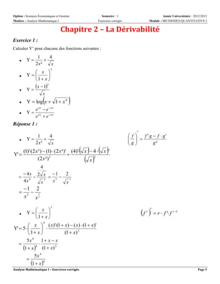
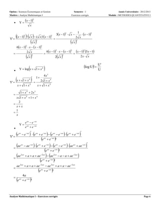
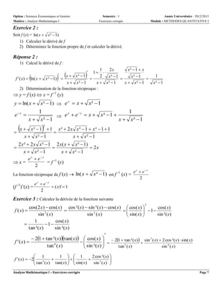
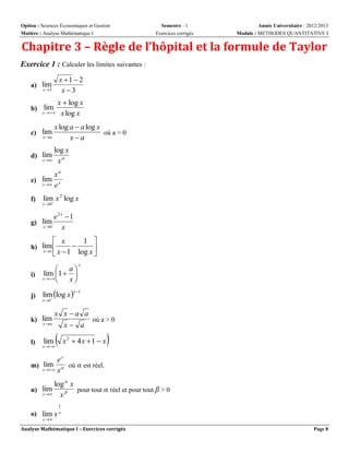
Option : Sciences Économiques et Gestion
Matière : Analyse Mathématique I

Semestre : 1
Exercices corrigés

Année Universitaire : 2012/2013
Module : METHODES QUANTITATIVE I

La Campagne Estudiantine pour Résumer
les Cours et Organiser les Polycopiés

Option : Science Economique et Gestion
Module : METHODES QUANTITATIVES I
Matière : Analyse Mathématique I
Semestre : 1
Type de document : Exercices corrigés

Année universitaire 2012-2013
Analyse Mathématique I – Exercices corrigés

Page 1
Option : Sciences Économiques et Gestion
Matière : Analyse Mathématique I

Semestre : 1
Exercices corrigés

Année Universitaire : 2012/2013
Module : METHODES QUANTITATIVE I

Chapitre 1 – La Continuité
Exercice 1 :
Déterminer le domaine de définition et les limites infinies de la fonction suivante :
( )

√

( )
Df = (

√

Réponse 1
)

( )
( )(
1 3
x1 
 2
2

–∞

x

)

–2



lim f ( x)  

x  

car

lim 2 x  1  

x 

lim f ( x)  lim 2 x  1  x²(1 

x 

x 

==> lim x(2 
x 

Car :

+

lim x²  x  2  

x

1 2

= lim 2 x  1  x x²  x  2
x x² x

1
1 2
 1   )  
x
x x²

lim x  

x 

et

+∞

1
–

+


==>
1 3
x2 
1
2

et

lim (2 

x 

1
1 2
 1  )  1
x
x x²

Exercice 2 :
Déterminer les domaines de définition et les domaines de continuité pour les fonctions définies par :

A. f ( x) 

x
x²  1

3x  1
B. f ( x)    x 1
e
Réponse 2
x
A. f ( x) 
x²  1

si x  1
si x  1

Df  x  IR / x²  1  0
Df  x  IR / x  1 ou x  1

Df  IR   1,1
DC  IR   1,1
Analyse Mathématique I – Exercices corrigés

Page 2
Option : Sciences Économiques et Gestion
Matière : Analyse Mathématique I

3x  
f ( x)    x1
B.
e

Semestre : 1
Exercices corrigés

Année Universitaire : 2012/2013
Module : METHODES QUANTITATIVE I

si x  1
si x  1
Df  IR

lim f ( x)  lim e x 1  e0  1
x 1

x 1

f (1)  3  
DC  IR
1
Soit λ ≠ – 2 : f est discontinue en 1 DC  IR   
Exercice 3 : Etudiez la continuité des fonctions suivantes :
Soit λ = – 2 : f est continue en 1

 2 x
si x  1

A. f ( x)   x  1
 2 x  1 si x  1






 x3  x 2  x 1

x 1
B. f ( x)  
 3 x


si x  1
si x  1

 x2  x  3  3
si x   3

x2  3
C. f ( x)  
 3x
si x   3


 x 1 1
si x  2 R  2

D. f ( x)   x  2
1
si x  2


Réponse 3 :
 2x
si x  1

A. f ( x)   x  1
si x  1

2 x 1






Si x = 1 ; f (1) = 1

Df = IR


Pour x  1 : lim f ( x)  lim 2  x  1  f (1)





Pour x > 1 : lim f ( x)  lim



x 1

x 1

 lim

x 1

x 1

x 1

x  1 x  1  lim 
x 1
2x  1






x  1 x  1
x 1
 lim

2 x  1 x1 2 x  1 x  1













x 1 11

 1  f (1)
2
2

f est continue au point 1
Analyse Mathématique I – Exercices corrigés

Page 3
Option : Sciences Économiques et Gestion
Matière : Analyse Mathématique I

 x3  x2  x  1

B. f ( x)  
x 1
 3 x



Semestre : 1
Exercices corrigés

Année Universitaire : 2012/2013
Module : METHODES QUANTITATIVE I

si x  1
si x  1

f (1)  2

x  1x 2  1
x3  x 2  x 1
x 2 x  1  x  1
 lim
 lim
x 1
x 1
x 1
x 1
x 1
x 1
2
 lim x  1  2  f (1)


Pour x < 1 : lim f ( x)  lim


x 1

x 1



Pour x ≥ 1 : lim f ( x)  lim


x 1

x 1

3 x 

3  1  2  f (1)

f est continue au point 1
x2  x  3  3
si x   3

C. f ( x)  
x2  3
4
si x   3



Pour x   3 : f ( x)

lim

x 

x 3





x 




3 1
  

x 3
x 3


x  3 1
lim 
  


x 3
x 3

f est continue sur IR   3, 3 .


lim





 

 



x2  x  3  3
x 3 x 3  x 3
x  3 1


2
x 3
x 3 x 3
x 3







3 1 2 3 1

 f ( 3)
x 3
2 3
 3  3 1 1
  
0 
 3 3

 3  3 1 1
  
0 
 3 3


















f est discontinue de 1er espèce non éliminable au point 3 .
f admet une discontinue de second espèce infinie au - 3
 x 1 1

D. f ( x)   x  2
1


si x  2 R  2
si x  2
Df   ,2  2,  2   ,
1
1







x 1 1
x 1 1 x 1  1
x2



x2
x  2 x  1  1
x  2 x  1  1
1
1
lim f ( x)  lim
  f (2)
x 2
x 2
2
x 1  1
f est continue sur 1,2  2,
f est discontinue de 1er espèce éliminable au point 2.
f admet un discontinuité de 1er espèce éliminable au point 2.


Pour x  2 : f ( x) 









 

1
x 1  1





Analyse Mathématique I – Exercices corrigés

Page 4
Option : Sciences Économiques et Gestion
Matière : Analyse Mathématique I

Semestre : 1
Exercices corrigés

Année Universitaire : 2012/2013
Module : METHODES QUANTITATIVE I

Chapitre 2 – La Dérivabilité
Exercice 1 :
Calculez Y’ pour chacune des fonctions suivantes :

1
4

2 x²
x



Y



 x 
Y

1 x 

5



x  13
Y



Y  log x  1  x 4



e ax  e  ax
Y  ax
e  e ax

x





Réponse 1 :


Y' 

1
4
Y

2 x²
x

   x '
 


f
f 'g  f  g '
  
g
g²
 

(1)'(2 x ²)  (1)  (2 x ²)' (4)' x  4 

2
(2 x ²) 2
x
4



 4x 2 x  1
2

 3 
4
2
3
4x
x
x
x



1 2
 3
x3 x 2



 x 
Y

1 x 

5

 f   r  f ' f
r

r 1

 x  ( x)'(1  x)  ( x)  (1  x)'
Y'  5  
 
(1  x) 2
1 x 
5x 4 1  x  x


4
1  x  (1  x) 2
5x 4

1  x 6
4

Analyse Mathématique I – Exercices corrigés

Page 5
Option : Sciences Économiques et Gestion
Matière : Analyse Mathématique I

x

x  1 ' x   (
 x

3



2

6x  1  x  x  1
2



2

3

2 x
2

6x  1  x  x  1

3

 

2 x



Y  log x  1  x

4

x  12 5x  1

2x  x

3

log U '  U'



U

4x3

x 
Y' 

1 x4

x  1 x4



 x  1

 x
2

 x



1

3

2 x



3x  1  x 
2

x )'x  1

3

Y' 

Année Universitaire : 2012/2013
Module : METHODES QUANTITATIVE I

x  13

Y



Semestre : 1
Exercices corrigés

  1  2 1  x

4

x  1 x4

1  x 4  2x3

x 1 x4 1 x4
2

xx
1

x
Y


e
Y' 

ax

e ax  e  ax
e ax  e ax



 e ax  e ax  e ax  e ax  e ax  e ax  e ax
e ax  e ax ²

 

ae


ax

ae


2 ax

 







 







 ae ax  e ax  e ax  e ax  e ax  ae ax  ae ax
e ax  e ax ²



 a  a  ae   ae  a  a  ae 
e  e ²
2 ax
ax

2 ax



2 ax

 ax

ae 2 ax  a  a  ae 2 ax  ae 2 ax  a  a  ae 2 ax
e ax  e ax ²
4a
 ax
e  e ax ²






Analyse Mathématique I – Exercices corrigés

Page 6
Option : Sciences Économiques et Gestion
Matière : Analyse Mathématique I

Semestre : 1
Exercices corrigés

Année Universitaire : 2012/2013
Module : METHODES QUANTITATIVE I

Exercice 2 :
Soit f (x) = ln( x  x²  1)
1) Calculez le dérivé de f
2) Déterminez la fonction propre de f et calculer la dérivé.

Réponse 2 :
1) Calcul le dérivé de f :

1
2x
x²  1  x


x  x²  1
2 x²  1
x²  1
f ' ( x)  ln( x  x ²  1) 



x  x²  1
x  x²  1
x  x²  1
2) Détermination de la fonction réciproque :

 







1

1
x²  1

 y = f (x)  x = f -1 (y)

y  ln( x  x²  1)  e y  x  x²  1

e y 

x 


1
1
y
y
 e  e  x  x²  1 
x  x²  1
x  x²  1



2

x²  1  1 x²  2 x x²  1  x²  1  1

x  x²  1
x  x²  1

2 x ²  2 x x ²  1 2 x ( x  x ²  1)

 2x
x  x²  1
x  x²  1
e y  e y
x=
= f -1 (y)
2


La fonction réciproque de f (x)  ln( x 

(f -1)’(x) =

e e
2
y

y

y
y
x²  1) est f -1 (x) = e  e

2

 ( x)'  1

Exercice 3 : Calculez la dérivée de la fonction suivante
2

cos(2 x)  cos( x) cos ²( x)  sin ²( x)  cos( x)  cos( x) 
cos( x)

f ( x) 

2
2
 sin( x)   1  sin ²( x)

sin ( x)
sin ( x)


1
cos( x)

1 
tan ²( x)
sin ²( x)

 21  tan ²( x) tan( x)   cos( x)   21  tan ²(x)  sin 3 ( x)  2 cos ²(x)  sin( x)
f ' ( x) 


 sin ²( x)  

tan 4 ( x)
tan 3 ( x)
sin 4 ( x)


 1
1   1
2 cos ²( x) 
f ' ( x)  2
 tan 3 ( x)  tan( x)    sin( x)  sin 3 ( x) 
 


 

Analyse Mathématique I – Exercices corrigés

Page 7
Option : Sciences Économiques et Gestion
Matière : Analyse Mathématique I

Semestre : 1
Exercices corrigés

Année Universitaire : 2012/2013
Module : METHODES QUANTITATIVE I

Chapitre 3 – Règle de l’hôpital et la formule de Taylor
Exercice 1 : Calculer les limites suivantes :
x 1  2
x 3

a) lim
x 3

x  log x
x   x log x

b) lim

x log a  a log x
où a > 0
xa

c) lim
x a

log x
x  x 

d) lim

x
e) lim x
x  e
f)

lim x 2 log x

x 0 

e2x 1
x

g) lim
x 0

 x
1 


 x  1 log x 

h) lim 
x 1

 a
i) lim 1  
x 
x

j)

lim log x 


x 1

x 1

k) lim
x a

l)

x

lim

x x a a
où a > 0
x a

x 

x

2

 4x  1  x



ex
m) lim  où α est réel.
x  x
log  x
n) lim
pour tout α réel et pour tout β > 0
x 
x
o) lim x

1
x

x 

Analyse Mathématique I – Exercices corrigés

Page 8
Option : Sciences Économiques et Gestion
Matière : Analyse Mathématique I

Semestre : 1
Exercices corrigés

Année Universitaire : 2012/2013
Module : METHODES QUANTITATIVE I

Réponse 1 :
a) lim
x 3



lim
x 3



x 1  2
x 3

Sans l’aide de règle de l’Hospital :

x 1  2
 lim
x 3
x3



x 1  2

x  3



x 1  2

x 1  2



  lim
x 3

x 1 4

x  3

x 1  2



 lim
x 3

1
x 1  2



1
4

Avec la règle de l’Hospital :

lim
x 3

Il vient que

x  1  2 R.H
lim
 lim
x 3
x 3
x 3

x  1  2 F.I 0

x3
0



x 1  2
x  3
1
 lim 2 x  1
x 3
1
1

4

(Forme Indéterminée de type

0
)
0



1
x  log x   lim
x  log x 
x
  lim
b) xlim

 x log x
x 
x  ( x )' (log x )  ( x )(log x )'

x log x 
1



1
x  1 0
 lim
 lim
x  
x   log x  1
1

log x  x 
x
1

1
x

1


 xlim log x   et
 

lim

x 

1

 0
x


x log a  a log x 
x log a  a log x 0
  lim
c) lim
x a
xa
0 x a
( x  a)'
( x)' (log a)  (a)' (log x)  (a)(log x)'
 lim
x a
x a
1 0

 lim

log a 
1

a
x  log a  1

log x
x  x 

Si α  0 : lim log x  x  
d) lim

x 

1
log x 
1
Si α > 0 : lim    lim x 1  lim   0

x  x
x  x
 x x
Analyse Mathématique I – Exercices corrigés

Page 9
Option : Sciences Économiques et Gestion
Matière : Analyse Mathématique I

e) lim
x 

Semestre : 1
Exercices corrigés

Année Universitaire : 2012/2013
Module : METHODES QUANTITATIVE I

x
ex

 Si α  0 : lim
x 
 Si α > 0 :

1
0
x  ex






 1

- si α  1 lim x x    lim ( x x )'  lim ax x  0
x 
x 
x 


e

(e )'

e

- si α > 1, on applique la règle de l’Hospital pour 2
D’après ces formules, on peut dire que xIR et α > 0.

lim x 2 log x  lim

f)

x 0

x 0

ème

(a 2  a)  x   2
0
fois : lim
x 
ex

si (α  2)

log x 

1

2
x

On applique la règle de l’Hospital :
1
1
log x   lim x  lim x  lim  x²  0
lim
 x 0   2 x x 0   2 x 0  2
x 0 
 1 
 2
x4
x3
x 

e2x 1 0
2e 2 x
  lim
 lim 2e 2 x  2
g) lim
x 0
x 0
x
0 x0 1
x

 a

h) lim 1   = 1
x 
 x
a
Si lim 1  a  = 1, alors ln 1  lim x log1    0  




x



x 

x

x  



x

 a
log1  
a
x


On peut la mettre sous forme 0 , car lim x log1    lim
x  
1
x  x 
0

x
En utilisant la règle de l’Hospital, cette limite est égale à :

a
x²
a
1
x  lim a  a
ln 1  lim
a
x  
x 
1
a
a
1
1
x
x


a


 0
 xlim
   


a
Par conséquent : 1  e

Analyse Mathématique I – Exercices corrigés

Page 10

S1 mqi-analysesmathmatiquesi-exercices

  • 1.
    Option : SciencesÉconomiques et Gestion Matière : Analyse Mathématique I Semestre : 1 Exercices corrigés Année Universitaire : 2012/2013 Module : METHODES QUANTITATIVE I La Campagne Estudiantine pour Résumer les Cours et Organiser les Polycopiés Option : Science Economique et Gestion Module : METHODES QUANTITATIVES I Matière : Analyse Mathématique I Semestre : 1 Type de document : Exercices corrigés Année universitaire 2012-2013 Analyse Mathématique I – Exercices corrigés Page 1
  • 2.
    Option : SciencesÉconomiques et Gestion Matière : Analyse Mathématique I Semestre : 1 Exercices corrigés Année Universitaire : 2012/2013 Module : METHODES QUANTITATIVE I Chapitre 1 – La Continuité Exercice 1 : Déterminer le domaine de définition et les limites infinies de la fonction suivante : ( ) √ ( ) Df = ( √ Réponse 1 ) ( ) ( )( 1 3 x1   2 2 –∞ x ) –2  lim f ( x)   x   car lim 2 x  1   x  lim f ( x)  lim 2 x  1  x²(1  x  x  ==> lim x(2  x  Car : + lim x²  x  2   x 1 2  = lim 2 x  1  x x²  x  2 x x² x 1 1 2  1   )   x x x² lim x   x  et +∞ 1 – +  ==> 1 3 x2  1 2 et lim (2  x  1 1 2  1  )  1 x x x² Exercice 2 : Déterminer les domaines de définition et les domaines de continuité pour les fonctions définies par : A. f ( x)  x x²  1 3x  1 B. f ( x)    x 1 e Réponse 2 x A. f ( x)  x²  1 si x  1 si x  1 Df  x  IR / x²  1  0 Df  x  IR / x  1 ou x  1 Df  IR   1,1 DC  IR   1,1 Analyse Mathématique I – Exercices corrigés Page 2
  • 3.
    Option : SciencesÉconomiques et Gestion Matière : Analyse Mathématique I 3x   f ( x)    x1 B. e Semestre : 1 Exercices corrigés Année Universitaire : 2012/2013 Module : METHODES QUANTITATIVE I si x  1 si x  1 Df  IR lim f ( x)  lim e x 1  e0  1 x 1 x 1 f (1)  3   DC  IR 1 Soit λ ≠ – 2 : f est discontinue en 1 DC  IR    Exercice 3 : Etudiez la continuité des fonctions suivantes : Soit λ = – 2 : f est continue en 1  2 x si x  1  A. f ( x)   x  1  2 x  1 si x  1     x3  x 2  x 1  x 1 B. f ( x)    3 x  si x  1 si x  1  x2  x  3  3 si x   3  x2  3 C. f ( x)    3x si x   3   x 1 1 si x  2 R  2  D. f ( x)   x  2 1 si x  2  Réponse 3 :  2x si x  1  A. f ( x)   x  1 si x  1  2 x 1    Si x = 1 ; f (1) = 1 Df = IR  Pour x  1 : lim f ( x)  lim 2  x  1  f (1)    Pour x > 1 : lim f ( x)  lim   x 1 x 1  lim  x 1 x 1 x 1 x  1 x  1  lim  x 1 2x  1    x  1 x  1 x 1  lim  2 x  1 x1 2 x  1 x  1       x 1 11   1  f (1) 2 2 f est continue au point 1 Analyse Mathématique I – Exercices corrigés Page 3
  • 4.
    Option : SciencesÉconomiques et Gestion Matière : Analyse Mathématique I  x3  x2  x  1  B. f ( x)   x 1  3 x   Semestre : 1 Exercices corrigés Année Universitaire : 2012/2013 Module : METHODES QUANTITATIVE I si x  1 si x  1 f (1)  2 x  1x 2  1 x3  x 2  x 1 x 2 x  1  x  1  lim  lim x 1 x 1 x 1 x 1 x 1 x 1 2  lim x  1  2  f (1)  Pour x < 1 : lim f ( x)  lim   x 1 x 1  Pour x ≥ 1 : lim f ( x)  lim   x 1 x 1 3 x  3  1  2  f (1) f est continue au point 1 x2  x  3  3 si x   3  C. f ( x)   x2  3 4 si x   3   Pour x   3 : f ( x) lim x  x 3   x    3 1     x 3 x 3   x  3 1 lim       x 3 x 3  f est continue sur IR   3, 3 .  lim        x2  x  3  3 x 3 x 3  x 3 x  3 1   2 x 3 x 3 x 3 x 3    3 1 2 3 1   f ( 3) x 3 2 3  3  3 1 1    0   3 3   3  3 1 1    0   3 3          f est discontinue de 1er espèce non éliminable au point 3 . f admet une discontinue de second espèce infinie au - 3  x 1 1  D. f ( x)   x  2 1  si x  2 R  2 si x  2 Df   ,2  2,  2   , 1 1    x 1 1 x 1 1 x 1  1 x2    x2 x  2 x  1  1 x  2 x  1  1 1 1 lim f ( x)  lim   f (2) x 2 x 2 2 x 1  1 f est continue sur 1,2  2, f est discontinue de 1er espèce éliminable au point 2. f admet un discontinuité de 1er espèce éliminable au point 2.  Pour x  2 : f ( x)        1 x 1  1   Analyse Mathématique I – Exercices corrigés Page 4
  • 5.
    Option : SciencesÉconomiques et Gestion Matière : Analyse Mathématique I Semestre : 1 Exercices corrigés Année Universitaire : 2012/2013 Module : METHODES QUANTITATIVE I Chapitre 2 – La Dérivabilité Exercice 1 : Calculez Y’ pour chacune des fonctions suivantes : 1 4  2 x² x  Y   x  Y  1 x  5  x  13 Y  Y  log x  1  x 4  e ax  e  ax Y  ax e  e ax x   Réponse 1 :  Y'  1 4 Y  2 x² x    x '    f f 'g  f  g '    g g²   (1)'(2 x ²)  (1)  (2 x ²)' (4)' x  4   2 (2 x ²) 2 x 4   4x 2 x  1 2   3  4 2 3 4x x x x  1 2  3 x3 x 2   x  Y  1 x  5  f   r  f ' f r r 1  x  ( x)'(1  x)  ( x)  (1  x)' Y'  5     (1  x) 2 1 x  5x 4 1  x  x   4 1  x  (1  x) 2 5x 4  1  x 6 4 Analyse Mathématique I – Exercices corrigés Page 5
  • 6.
    Option : SciencesÉconomiques et Gestion Matière : Analyse Mathématique I x x  1 ' x   (  x 3  2 6x  1  x  x  1 2  2 3 2 x 2 6x  1  x  x  1 3   2 x  Y  log x  1  x 4 x  12 5x  1  2x  x 3 log U '  U'  U 4x3 x  Y'  1 x4 x  1 x4   x  1  x 2  x  1 3 2 x  3x  1  x  2 x )'x  1 3 Y'  Année Universitaire : 2012/2013 Module : METHODES QUANTITATIVE I x  13 Y  Semestre : 1 Exercices corrigés   1  2 1  x 4 x  1 x4 1  x 4  2x3 x 1 x4 1 x4 2  xx 1  x Y  e Y'  ax e ax  e  ax e ax  e ax    e ax  e ax  e ax  e ax  e ax  e ax  e ax e ax  e ax ²   ae  ax ae  2 ax            ae ax  e ax  e ax  e ax  e ax  ae ax  ae ax e ax  e ax ²    a  a  ae   ae  a  a  ae  e  e ² 2 ax ax 2 ax  2 ax  ax ae 2 ax  a  a  ae 2 ax  ae 2 ax  a  a  ae 2 ax e ax  e ax ² 4a  ax e  e ax ²    Analyse Mathématique I – Exercices corrigés Page 6
  • 7.
    Option : SciencesÉconomiques et Gestion Matière : Analyse Mathématique I Semestre : 1 Exercices corrigés Année Universitaire : 2012/2013 Module : METHODES QUANTITATIVE I Exercice 2 : Soit f (x) = ln( x  x²  1) 1) Calculez le dérivé de f 2) Déterminez la fonction propre de f et calculer la dérivé. Réponse 2 : 1) Calcul le dérivé de f : 1 2x x²  1  x   x  x²  1 2 x²  1 x²  1 f ' ( x)  ln( x  x ²  1)     x  x²  1 x  x²  1 x  x²  1 2) Détermination de la fonction réciproque :      1 1 x²  1  y = f (x)  x = f -1 (y) y  ln( x  x²  1)  e y  x  x²  1 e y  x   1 1 y y  e  e  x  x²  1  x  x²  1 x  x²  1  2 x²  1  1 x²  2 x x²  1  x²  1  1  x  x²  1 x  x²  1 2 x ²  2 x x ²  1 2 x ( x  x ²  1)   2x x  x²  1 x  x²  1 e y  e y x= = f -1 (y) 2  La fonction réciproque de f (x)  ln( x  (f -1)’(x) = e e 2 y y y y x²  1) est f -1 (x) = e  e 2  ( x)'  1 Exercice 3 : Calculez la dérivée de la fonction suivante 2 cos(2 x)  cos( x) cos ²( x)  sin ²( x)  cos( x)  cos( x)  cos( x)  f ( x)   2 2  sin( x)   1  sin ²( x)  sin ( x) sin ( x)   1 cos( x)  1  tan ²( x) sin ²( x)   21  tan ²( x) tan( x)   cos( x)   21  tan ²(x)  sin 3 ( x)  2 cos ²(x)  sin( x) f ' ( x)     sin ²( x)    tan 4 ( x) tan 3 ( x) sin 4 ( x)    1 1   1 2 cos ²( x)  f ' ( x)  2  tan 3 ( x)  tan( x)    sin( x)  sin 3 ( x)         Analyse Mathématique I – Exercices corrigés Page 7
  • 8.
    Option : SciencesÉconomiques et Gestion Matière : Analyse Mathématique I Semestre : 1 Exercices corrigés Année Universitaire : 2012/2013 Module : METHODES QUANTITATIVE I Chapitre 3 – Règle de l’hôpital et la formule de Taylor Exercice 1 : Calculer les limites suivantes : x 1  2 x 3 a) lim x 3 x  log x x   x log x b) lim x log a  a log x où a > 0 xa c) lim x a log x x  x  d) lim x e) lim x x  e f) lim x 2 log x x 0  e2x 1 x g) lim x 0  x 1     x  1 log x  h) lim  x 1  a i) lim 1   x  x  j) lim log x   x 1 x 1 k) lim x a l) x lim x x a a où a > 0 x a x  x 2  4x  1  x  ex m) lim  où α est réel. x  x log  x n) lim pour tout α réel et pour tout β > 0 x  x o) lim x 1 x x  Analyse Mathématique I – Exercices corrigés Page 8
  • 9.
    Option : SciencesÉconomiques et Gestion Matière : Analyse Mathématique I Semestre : 1 Exercices corrigés Année Universitaire : 2012/2013 Module : METHODES QUANTITATIVE I Réponse 1 : a) lim x 3  lim x 3  x 1  2 x 3 Sans l’aide de règle de l’Hospital : x 1  2  lim x 3 x3  x 1  2 x  3  x 1  2 x 1  2    lim x 3 x 1 4 x  3 x 1  2   lim x 3 1 x 1  2  1 4 Avec la règle de l’Hospital : lim x 3 Il vient que x  1  2 R.H lim  lim x 3 x 3 x 3 x  1  2 F.I 0  x3 0  x 1  2 x  3 1  lim 2 x  1 x 3 1 1  4 (Forme Indéterminée de type 0 ) 0  1 x  log x   lim x  log x  x   lim b) xlim   x log x x  x  ( x )' (log x )  ( x )(log x )'  x log x  1  1 x  1 0  lim  lim x   x   log x  1 1  log x  x  x 1 1 x 1   xlim log x   et   lim x  1   0 x  x log a  a log x  x log a  a log x 0   lim c) lim x a xa 0 x a ( x  a)' ( x)' (log a)  (a)' (log x)  (a)(log x)'  lim x a x a 1 0  lim log a  1 a x  log a  1 log x x  x   Si α  0 : lim log x  x   d) lim x  1 log x  1 Si α > 0 : lim    lim x 1  lim   0  x  x x  x  x x Analyse Mathématique I – Exercices corrigés Page 9
  • 10.
    Option : SciencesÉconomiques et Gestion Matière : Analyse Mathématique I e) lim x  Semestre : 1 Exercices corrigés Année Universitaire : 2012/2013 Module : METHODES QUANTITATIVE I x ex  Si α  0 : lim x   Si α > 0 : 1 0 x  ex     1 - si α  1 lim x x    lim ( x x )'  lim ax x  0 x  x  x   e (e )' e - si α > 1, on applique la règle de l’Hospital pour 2 D’après ces formules, on peut dire que xIR et α > 0. lim x 2 log x  lim f) x 0 x 0 ème (a 2  a)  x   2 0 fois : lim x  ex si (α  2) log x   1  2 x On applique la règle de l’Hospital : 1 1 log x   lim x  lim x  lim  x²  0 lim  x 0   2 x x 0   2 x 0  2 x 0   1   2 x4 x3 x  e2x 1 0 2e 2 x   lim  lim 2e 2 x  2 g) lim x 0 x 0 x 0 x0 1 x  a  h) lim 1   = 1 x   x a Si lim 1  a  = 1, alors ln 1  lim x log1    0       x  x  x x    x  a log1   a x   On peut la mettre sous forme 0 , car lim x log1    lim x   1 x  x  0  x En utilisant la règle de l’Hospital, cette limite est égale à : a x² a 1 x  lim a  a ln 1  lim a x   x  1 a a 1 1 x x  a    0  xlim      a Par conséquent : 1  e Analyse Mathématique I – Exercices corrigés Page 10