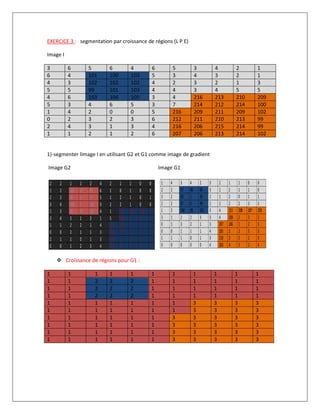
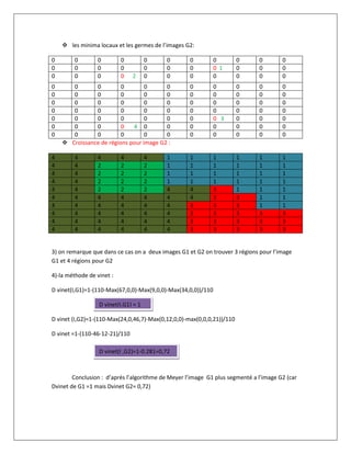
Le document décrit le traitement d'image à travers l'égalisation d'histogramme, l'application de filtres gaussiens et la détection de contours avec divers opérateurs. Il fournit également un exercice sur la segmentation par croissance de régions et introduit la méthode de Vinet pour évaluer la qualité de segmentation. Les résultats montrent que g1 est mieux segmenté que g2 selon l'algorithme de Meyer.

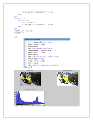
![Egalisation d’histogramme :
Pour généraliser l’égalisation l’histogramme au cas d’une image couleur il faut
respecter les quatre étapes suivantes :
1. Calcule de l’intensité de l’image couleur I=(R+V+B)/3.
2. Calcule de l’histogramme de I.
3. Calcule de l’histogramme cumulé de I.
4. l’égalisation de l’histogramme dans chaque l’image couleur ?
le programme de l’égalisation une image couleur est :
function C=egalisationcouleur(I);
[w,h,c]=size(I);
if c==3
R=I(:,:,1);
G=I(:,:,2);
B=I(:,:,3);
I=(R+G+B)./3;
end
J=double(I);
H=zeros(256);
HC=zeros(256);
% on peut utilisetr taille=numel(I)
for m=1:w
for n= 1:h
val=J(m,n);
H(val+1)=H(val+1)+1;
end
end
% calcul de l'histogramme cumulé
HC(1)=H(1);
for m= 2:256
HC(m)=(HC(m-1)+H(m));
end
%transformtion de l'image
for m= 1:w
for n= 1:h
val = R(m,n);
C1(m,n)=255*HC(val+1)/(w*h);
end
end
for m= 1:w
for n= 1:h
val = G(m,n);](https://image.slidesharecdn.com/el-anza-1-170107174511/85/devoir-traitement-d-images-2-320.jpg)
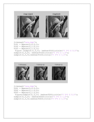
![3 :: Implémenter la fonction Ngauss qui retourne le noyau gaussian
dont la taille et la valeur de sigma sont passées en entrée.
function [J] = Ngauss(I,sigma,taille)
switch taille
case 1
disp('taille 3*3');
[x,y]=meshgrid(-1:1,-1:1);
case 2
disp('taille 5*5');
[x,y]=meshgrid(-2:2,-2:2);
case 3
disp('taille 7*7');
[x,y]=meshgrid(-3:3,-3:3);
end
G=(1/(2*pi*(sigma)^2))*exp(-(x.^2+y.^2)/(2*sigma^2));
J=imfilter(I,G);
J=uint8(J);
imshow(J);
end
I=imread(‘lena.bmp');
J = imnoise(I,'gaussian');
subplot(1,2,1);imshow(I);title('imageoriginal');
subplot(1,2,2);imshow(J);title('imagebruité');](https://image.slidesharecdn.com/el-anza-1-170107174511/85/devoir-traitement-d-images-4-320.jpg)
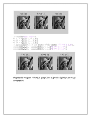
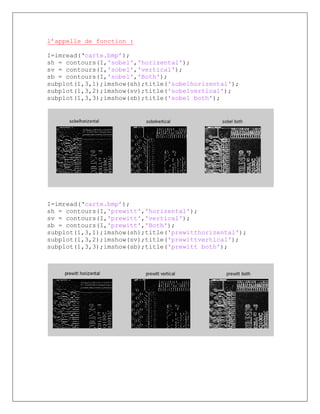
![La détection de contours avec sobel et prewitt :
function g= contours(I,operateur,direction)
J=double(I);
switch operateur
case 'sobel'
Sx=[-1 -2 -1 ;0 0 0;1 2 1];
Sy=Sx';
case 'prewitt'
Sx=[-1 -1 -1 ;0 0 0;1 1 1];
Sy=Sx';
end
switch direction
case 'horizental'
g=filter(J,Sx);
case 'vertical'
g=filter(J,Sy);
case 'Both'
Gx=filter(J,Sx);
Gy=filter(J,Sy);
g=sqrt(Gx.^2+Gy.^2);
end
g=uint8(g);
imshow(g);
function k=filter(f,o)
[w,h]=size(f);
k=zeros(w,h);
for l=2:w-1
for c=2:h-1
K=o.*f(l-1:l+1,c-1:c+1);
k(l,c)=sum(K(:));
end
end
end
end](https://image.slidesharecdn.com/el-anza-1-170107174511/85/devoir-traitement-d-images-7-320.jpg)