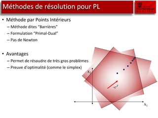
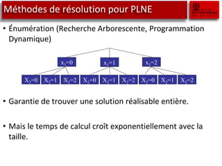
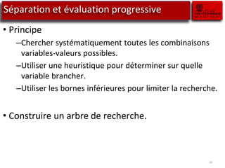
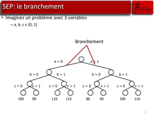
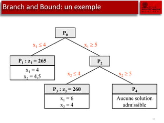
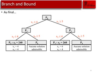
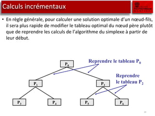
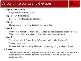
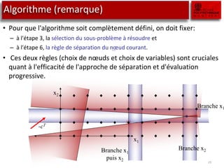
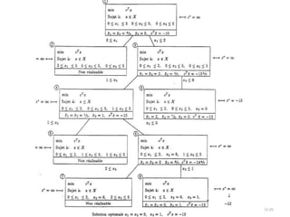
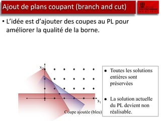
Le document traite des outils de recherche opérationnelle, en particulier sur la programmation en nombre entier (PLNE) et les méthodes de résolution telles que le simplexe et le branch and bound. Il explique comment ces méthodes sont appliquées pour résoudre des problèmes d'optimisation en utilisant des techniques telles que la relaxation linéaire et les sous-problèmes. Des astuces de modélisation pour des cas complexes, tels que les coûts fixes et les contraintes conditionnelles, sont également abordées.

1. Outils de Recherche
opérationnelle en Génie MTH
8414
Programmation en nombre entier:
Méthode de résolution et astuces de modélisation

2. Types de problème d’optimisation
• Programme Linéaire en Nombre Entier (PLNE ou IP) :
• Programme Linéaire en Nombre Entier Mix (MIP) :
• Ces problèmes sont théoriquement très difficiles, mais en
pratique ils peuvent (souvent) être résolus très rapidement.

3. 3
Formulation PLNE
X
on obtient un PL nommé
“Relaxation Linéaire”
• Résolu par séparation et évaluation progressive
– on branche sur les variables de décision
– la relaxation linéaire nous donne des bornes inférieures.

4. Méthodes de résolution pour PL
• Algorithme du simplex
– Une solution optimale se trouve nécessairement sur un point extrême.
– Donc on peut la trouver en parcourant les arêtes du polyèdre.
cT
x1
x2

5. Méthodes de résolution pour PL
• Méthode par Points Intérieurs
– Méthode dites “Barrières”
– Formulation “Primal-Dual”
– Pas de Newton
• Avantages
– Permet de résoudre de très gros problèmes
– Preuve d’optimalité (comme le simplex)
-cT
x1
x2

6. Méthodes de résolution pour PLNE
• Énumération (Recherche Arborescente, Programmation
Dynamique)
• Garantie de trouver une solution réalisable entière.
• Mais le temps de calcul croît exponentiellement avec la
taille.
x1=0
X2=0 X2=2
X2=1
x1=1 x1=2
X2=0 X2=2
X2=1
X2=0 X2=2
X2=1

7. Méthodes de résolution pour PLNE
• Résoudre un PL puis arrondir ?
-cT
x1
x2
Solution du PL
Solution entière

8. Méthodes de résolution pour PLNE
• Le PL fournit une borne inf (ou sup si on maximise) sur la valeur
du PLNE.
• Mais en arrondissant, on peut être très loin d’une solution
entière…
-cT
x1
x2

9. Approche combinée pour PLNE.
• On peut combiner les deux approches
– Résoudre le PL pour obtenir une solution.
– Créer deux sous-problèmes en ajoutant des
contraintes.
-cT
x1
x2
-cT
x1
x2
x1≤1
x1≥2

10. 10
Séparation et évaluation progressive
• Principe
–Chercher systématiquement toutes les combinaisons
variables-valeurs possibles.
–Utiliser une heuristique pour déterminer sur quelle
variable brancher.
–Utiliser les bornes inférieures pour limiter la recherche.
• Construire un arbre de recherche.

11. 11
SEP: le branchement
• Imaginez un problème avec 3 variables
– a, b, c є {0, 1}
a = 0 a = 1
b = 0 b = 1
c = 0 c = 1 c = 0 c = 1 c = 0 c = 1
c = 0 c = 1
b = 0 b = 1
100 90 110 115 80 90 100 110
Branchement

12. 12
SEP: utilisation des bornes inférieures
• Si nous pouvions calculer une borne sur le coût minimal d’un noeud.
a = 0 a = 1
b = 0 b = 1
c = 0 c = 1 c = 0
b = 0
100 90 80
50
70
85 95
80
80

13. 13
Séparation et évaluation progressive
• Mieux connu sous le nom anglais “branch and bound”
• Branch: assigne heuristiquement une valeur à une variable
–Crée deux sous problèmes
• Bound: comparer la borne inférieure à la meilleure solution
connue
–Ça ne vaut pas la peine d’explorer le sous-arbre si
• Minimisation: si BorneInf >= MeilleureSolution,
• Maximisation: si BorneSup <= MeilleureSolution,

14. 14
SÉP pour résoudre des PLNE
• Généralement la borne inférieure = la relaxation linéaire.
– On l’obtient en « relaxant » les contraintes d’intégrité.
• On choisit une variable non entière et on la force soit à :
– être plus grande ou égale à l’entier supérieur ou
– être plus petite ou égale à l’entier inférieur.

15. Branch and Bound: un exemple
15
entiers
,
0
,
8
14
2
5
2
s.c.
50
10
max
2
1
2
1
1
2
1
2
1
2
1
x
x
x
x
x
x
x
x
x
x
x
z









Relaxation linéaire (ou continue)

16. Branch and Bound: un exemple
16
P0 : z0 = 282,5
x1 = 4,5
x2 = 4,75
Premier noeud
(solution optimale de la relaxation linéaire)
Valeur optimale
Variables non nulles

17. Branch and Bound
17
P1 : z1 = 265
x1 = 4
x2 = 4,5
P2 : z2 = 275
x1 = 5
x2 = 4,5
P0 noeud-père
noeuds-fils
x1  5
x1  4

18. Branch and Bound: un exemple
18
P1 : z1 = 265
x1 = 4
x2 = 4,5
P3 : z3 = 260
x1 = 6
x2 = 4
P0
x1  5
x1  4
P2
x2  5
x2  4
P4
Aucune solution
admissible

19. Branch and Bound
• Au final…
19
P5 : z5 = 240
x1 = 4
x2 = 4
P3 : z3 = 260
x1 = 6
x2 = 4
P0
x1  5
x1  4
P2
x2  5
x2  4
P4
Aucune solution
admissible
P1
P6
Aucune solution
admissible
x2  5
x2  4

20. Calculs incrémentaux
• En règle générale, pour calculer une solution optimale d’un nœud-fils,
il sera plus rapide de modifier le tableau optimal du nœud père plutôt
que de reprendre les calculs de l’algorithme du simplexe à partir de
leur début.
20
P0
P2
P1
P3 P4 P5 P6
Reprendre le tableau P0
Reprendre
le tableau P2

21. Algorithme (problème de minimisation)
21
Les notations suivantes sont utilisées :
L : ensemble des sous-problèmes actifs;
zU : la borne supérieure sur la valeur optimale de MIP ;
zi
LP : la valeur optimale du problème linéaire i ;
zj
LP : la borne inférieure sur la valeur optimale du sous-problème j ;
X* : La meilleure solution réalisable.

22. L'algorithme comprend 6 étapes :
– Étape 1 : Initialisation
L = {relaxation initiale}, zU = .
– Étape 2 : Test d'optimalité
Si L =  , x* est la solution optimale.
– Étape 3
Choisir un sous-problème i et l'éliminer de la liste L.
– Étape 4
Résoudre la relaxation linéaire de i. Si elle n'est pas réalisable, allez à l'étape 3
Sinon, poser zi
LP et xi la valeur et la solution optimales obtenues.
– Étape 5
Si zi
LP  zU , aller à l'étape 2. Si xi n'est pas entière, aller à l'étape 6.
Sinon zU = zi
LP, x* = xi.
Éliminer de L tous les sous-problèmes j tels que zj
LP  zU et aller à l'étape 2.
– Étape 6
Choisir une variable binaire ayant une valeur fractionnaire dans la solution xi et
subdiviser le problème i à partir de cette variable. Ajouter les nouveaux
problèmes à L.
22

23. Algorithme (remarque)
• Pour que l'algorithme soit complètement défini, on doit fixer:
– à l'étape 3, la sélection du sous-problème à résoudre et
– à l'étape 6, la règle de séparation du nœud courant.
• Ces deux règles (choix de nœuds et choix de variables) sont cruciales
quant à l'efficacité de l'approche de séparation et d'évaluation
progressive.
23
-cT
x1
x2
Branche x2
Branche x1
puis x2
Branche x1

24. Un autre exemple
• Soit le problème de PLNE suivant:
• Et la notation
24
entières.
et
0
,
,
5
5
5
8
7
3
6
8
7
6
3
:
à
sujet
13
3
3
min
:
)
(
3
2
1
3
2
1
3
2
1
3
2
1
3
2
1















x
x
x
x
x
x
x
x
x
x
x
x
x
x
x
z
P
3
2
1 13
3
3 x
x
x
x
c
z T





 
8
7
3
6
,
8
7
6
3
: 3
2
1
3
2
1
3








 x
x
x
x
x
x
I
x
X

25. 11-25

26. Ajout de plans coupant (branch and cut)
• L’idée est d’ajouter des coupes au PL pour
améliorer la qualité de la borne.
x1
x2
Coupe ajoutée (bleu)
 Toutes les solutions
entières sont
préservées
 La solution actuelle
du PL devient non
réalisable.

27. Trucs et astuces de modélisation
• Comment modéliser les cas où l’on est en présence de:
– variables ont des domaines discontinus;
– certaines ressources qui ont des coûts fixes;
– disjonctions de contraintes;
– contraintes conditionnelles
– de SOS et des fonctions linéaires par morceaux
– des produits de variables
27

28. Variables avec domaines discontinues
• Que faire avec le cas où soit x = 0 OU l <= x <= u
• On peut considérer ceci comme deux contraintes, mais elles ne
peuvent être vraies toutes les deux à la fois…
• Pouvez-vous trouver des exemples d’applications ?
• Comment modéliser ceci avec un PLNE ?
28
x = 0 or l ≤ x ≤ u
This can be interpreted as two constraints that cannot both hold simultane
ously. In linear programming only simultaneous constraints can be modeled.
0 l u
x
Figure 7.1: A discontinuous variable
This situation occurs when a supplier of some item requires that if an item
is ordered, then its batch size must be between a particular minimum and
maximum value. Another possibility is that there is a set-up cost associated
with the manufacture of an item.

29. Les coûts fixes
• Soit le problème suivant:
• La fonction de coût n’est ni linéaire ni continue...
• À quelle application pensez-vous ?
• Comment résoudre ce problème ?
30
model A fi xed cost problem is another application where indicator variables are ad
so that two mutually exclusive situations can be modeled. An examp
provided using a single-variable. Consider the following linear programm
model (the sign “≷” denotes either “≤ ”, “= ”, or “≥ ” constraints).
Minimize: C(x )
Subject to:
a i x +
j ∈ J
a i j w j ≷ bi ∀ i ∈ I
x ≥ 0
w j ≥ 0 ∀ j ∈ J
Where: C(x ) =
0 for x = 0
k + cx for x > 0
As soon as x has a positive value, a fi xed cost is incurred. This cost func
is not linear and is not continuous. There is a jump at x = 0, as illustrate
Figure 7.2.
lication In the above formulat ion, the discontinuous function is the objective, but
a function might equally well occur in a constraint. An example of su
fi xed-cost problem occurs in the manufacturing industry when set-up c
7.3. Either
C(x)
k
0 x
c

30. Une disjonction de contrainte
• Soit le problème suivant:
• Où soit (1) ou (2) doit être respectée
• Des applications ?
• Comment faire ?
32
7.3 Either-or constraints
The mod
Consider the following linear programming model:
Minimize:
j ∈J
cj x j

31. Contraintes conditionnelles
• Une variante de ce problème survient lorsque certaines contraintes
sont conditionnelles:
• Donnez des exemples d’application ?
• Comment traiter ce cas ?
34
A problem that can be treated in a similar way to either-or constraints is one
that contains conditional constraints. The mathematical presentation is lim-
ited to a case, involving two constraints, on which the following condition is
imposed.
If (1) (
j ∈ J
a 1j x j ≤ b1) is satisfied,
then (2) (
j ∈ J
a 2j x j ≤ b2) must also be satisfied.
Let A denote the statement that the logical expression “Constraint (1) holds”
is true, and similarly, let B denote the statement that the logical expression
“Constraint (2) holds” is true. The notation ¬ A and ¬ B represent the case
of the corresponding logical expressions being false. The above conditional
constraint can be restated as: A implies B. This is logically equivalent to writing
(A and ¬ B) is false. Using the negation of this expression, it follows that ¬ (A
and ¬ B) is true. This is equivalent to (¬ A or B) is true, using Boolean algebra.
It is this last equivalence that allows one to translate the above conditional
constraint into an either-or constraint.

32. Les SOS (Special Ordered Sets)
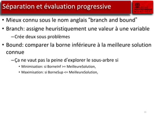
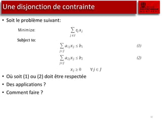
• Considérer le cas particulier suivant:
– Votre modèle comporte une série de décision oui/non ordonnée.
– Seulement une décision « oui » est possible
– Entre deux décisions « oui » on préfèrera toujours celle qui est la première dans la
série.
• Pour ce cela, on dispose généralement d’une série de variables booléennes
yi telles que
• On peut généraliser ce cas à :
– Aux variables générales xi tel que 0 <= xi <= u et sujet à
• On peut aussi considérer le cas où deux décisions « oui » sont permises,
mais elles doivent être consécutives.
• Les solveurs ont des objets de modélisation SOS1 et SOS2 qui implémentent
ces conditions de manières plus efficaces lors du branch and bound.
37
solvers. Two of them are treated in this section, and are re
cial Ordered Sets (SOS) of type 1 and 2. These concepts are
Tomlin ([Be69]).
SOS1
constraints
A common restriction is that out of a set of yes-no decisi
decision variable can be yes. You can model this as follow
zero-one variables, then
i
y i ≤ 1
forms an example of a SOS1 constraint. More generally, w
variables 0 ≤ x i ≤ u i , then the constraint
i
ai x i ≤ b
can also become a SOS1 constraint by adding the requirem
one of the x i can be nonzero. In Aimms there is a constrain
P
ropert yin which you can indicate whether this constraint is a
Note that in the general case, the variables are no longer rest
one variables.
lar types of restrictions in integer programming formulations
ommon, and that can be treated in an efficient manner by
them are treated in this section, and are referred to as Spe-
(SOS) of type 1 and 2. These concepts are due to Beale and
iction is that out of a set of yes-no decisions, at most one
can be yes. You can model this as follows. Let y i denote
es, then
i
y i ≤ 1
le of a SOS1 constraint. More generally, when considering
≤ u i , then the constraint
i
ai x i ≤ b
a SOS1 constraint by adding the requirement that at most
n be nonzero. In Aimms there is a constraint attribute named
you can indicate whether this constraint is a SOS1 constraint.
general case, the variables are no longer restricted to be zero-

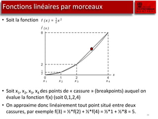
33. Fonctions linéaires par morceaux
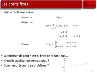
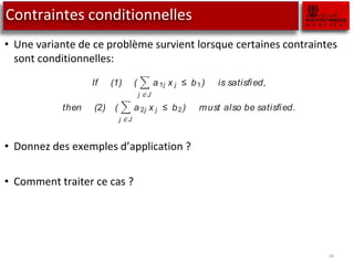
• Soit le problème suivant:
• Ici on remarque que l’objective, bien que non linéaire, est séparable.
• C’est-à-dire que l’objectif est une somme de fonctions définies sur
une variable à la fois.
Séparable Non séparable
38
7.6 Piecewise linear formulations
Consider the following model with a separable objective function:
Minimize:
j ∈ J
f j (x j )
Subject to:
j ∈ J
ai j x j ≷ bi ∀ i ∈ I
x j ≥ 0 ∀ j ∈ J
In the above general model statement, the objective is a separable function,
which is defi ned as the sum of functions of scalar variables. Such a func-
tion has the advantage that nonlinear terms can be approximated by piecewise
linear ones. Using this technique, it may be possible to generate an integer pro-
gramming model, or sometimes even a linear programming model (see [Wi90]).
This possibility also exists when a constraint is separable.
Some examples of separable functions are:
x 2
1 + 1/ x 2 − 2x 3 = f 1(x 1) + f 2(x 2) + f 3(x 3)
x 2
1 + 5x 1 − x 2 = g1(x 1) + g2(x 2)
The model
llowing model with a separable objective function:
j ∈ J
f j (x j )
j ∈ J
ai j x j ≷ bi ∀ i ∈ I
x j ≥ 0 ∀ j ∈ J
Separ able
function
eneral model statement, the objective is a separable function,
ed as the sum of functions of scalar variables. Such a func-
vantage that nonlinear terms can be approximated by piecewise
ng this technique, it may be possible to generate an integer pro-
el, or sometimes even a linear programming model (see [Wi90]).
also exists when a constraint is separable.
Examples of
separable
functions
of separable functions are:
x 2
1 + 1/ x 2 − 2x 3 = f 1(x 1) + f 2(x 2) + f 3(x 3)
x 2
1 + 5x 1 − x 2 = g1(x 1) + g2(x 2)
84 Chapter 7. Integer Linear Programming Tricks
The following examples are not:
x 1x 2 + 3x 2 + x 2
2 = f 1(x 1, x 2) + f 2(x 2)
1/ (x 1 + x 2) + x 3 = g1(x 1, x 2) + g2(x 3)
Approximation Consider a simple example with only one nonlinear term to b

34. Fonctions linéaires par morceaux
• Soit la fonction
• Soit x1, x2, x3, x4 des points de « cassure » (breakpoints) auquel on
évalue la fonction f(x) (soit 0,1,2,4)
• On approxime donc linéairement tout point situé entre deux
cassures, par exemple f(3) = ½*f(2) + ½*f(4) = ½*1 + ½*8 = 5. 39
1/ (x 1 + x 2) + x 3 = g1(x 1, x 2) + g2(x 3)
roximation
nonlinear
ction
Consider a simple example with only one nonlinear term to be approxima
namely f (x ) =
1
2 x 2
. Figure 7.3, shows the curve divided into three pieces
are approximated by straight lines. This approximation is known as piecew
linear. The points where the slope of the piecewise linear function changes
its domain ends) are referred to as breakpoints. This approximation can be
pressed mathematically in several ways. A method known as the λ-formula
is described below.
x
˜
f (x )
0 1 2 4
1
2
2
8
linear. The points where the slope of the piecewise linear function changes (or
its domain ends) are referred to as breakpoints. This approximation can be ex-
pressed mathematically in several ways. A method known as the λ -formulation
is described below.
x
˜
f (x )
0
x 1
1
x 2
2
x 3
4
x 4
1
2
2
8
Figure 7.3: Piecewise linear approximation of f (x ) = 1
2 x 2
ms Let x 1, x 2, x 3 and x 4 denote the four breakpoints along the x-axis in Figure 7.3,
and let f (x 1), f (x 2), f (x 3 ) and f (x 4) denote the corresponding function val-
ues. The breakpoints are 0, 1, 2 and 4, and the corresponding function values
are 0, 1
2 , 2 and 8. Any point in between two breakpoints is a weighted sum of

35. Fonctions linéaires par morceaux
• Une des manières de traiter ces fonctions est d’utiliser la λ-
formulation.
• Soit λ1, λ2, λ3, λ4, 4 poids non négatifs dont la somme = 1, alors la
fonction linéaire par morceaux précédente peut-être exprimée par:
• Comme au plus deux λ peuvent être non négatifs, et que ceux-ci
doivent en plus être consécutifs, on peut ajouter une contrainte
SOS2(λ).
• La majorité des solveurs ont un objet « Piecewise Linear » que vous
pouvez utiliser directement.
40
ues. The breakpoints are 0, 1, 2 and 4, and the corresponding function values
are 0,
1
2 , 2 and 8. Any point in between two breakpoints is a weighted sum of
hese two breakpoints. For instance, x = 3 =
1
2 · 2 +
1
2 · 4. The corresponding
approximated function value ˜
f (3) = 5 =
1
2
· 2 +
1
2
· 8.
Let λ 1, λ2, λ3, λ 4 denote four nonnegative weights such that their sum is 1.
Then the piecewise linear approximation of f (x ) in Figure 7.3 can be written
as:
λ1f (x 1) + λ2f (x 2) + λ3f (x 3) + λ4f (x 4) = ˜
f (x )
λ1x 1 + λ2x 2 + λ3x 3 + λ4x 4 = x
λ1 + λ 2 + λ3 + λ 4 = 1
with the added requirement that at most two adjacent λ’s are greater than
zero. This requirement together with the last constraint form the SOS2 con-

36. Éliminer les produits de variables
• Que faire des problèmes où des termes contiennent le produit de
deux variables booléennes x1x2
• On peut faire disparaître ce produit en introduisant une nouvelle
variable booléenne y qui doit être égale au produit x1x2.
• Pour ce faire il faut ajouter les contraintes suivantes:
41
a product of two variables can be replaced by one new variable, on
mber of constraints is imposed. The extension to products of more
variables is straightforward. Three cases are distinguished. In the
a separable function results (instead of a linear one) that can then
mated by using the methods described in the previous section.
nsider the binary variables x 1 and x 2. Their product, x 1x 2, can be
y an additional binary variable y . The following constraints force y
value of x 1x 2:
y ≤ x 1
y ≤ x 2
y ≥ x 1 + x 2 − 1
y binary

37. Excercise de modélisation
• On veut assembler l’horaire hebdomadaire de travail d’une unité d’infirmières
sachant que:
– On a trois quarts de 8h de travail à couvrir (J,S,N)
– Le nombre d’infirmières requises de dq où q est un quart de travail (J,S,N)
– Une infirmière doit avoir 16h de repos entre deux quarts.
• Les contraintes suivantes doivent être respectées
– Si on emploie une infirmière pendant la semaine, elle doit travailler au moins 3 quarts.
– Une infirmière doit avoir congé soit
• a) toutes les nuits de la semaine
• b) toute la fin de semaine.
– Si une infirmière travaille 4 quarts de travaille, elle doit avoir congé la fin de semaine.
– Chaque infirmière donne une liste de jours de congé souhaitée (et ordonnées), on doit lui
donner au moins un de ces choix.
• Il faut minimiser les coûts sachant que:
1. Si on emploie une infirmière il faut payer l’agence un montant fixe de F$ + G$ par quart
travaillé.
2. En plus, il est permis de ne pas avoir le bon nombre d’infirmières, mais il faut payer une
pénalité de P(k) $ ou k est la différence entre le nombre souhaité le nombre d’infirmières
assignées
43